ANOVA, MANOVA, and ANCOVA using R

Introduction

This tutorial introduces three closely related statistical methods for analysing differences between groups: ANOVA (Analysis of Variance), MANOVA (Multivariate Analysis of Variance), and ANCOVA (Analysis of Covariance). All three extend the logic of the t-test — which compares two group means — to more complex research designs involving multiple groups, multiple outcome variables, or the need to control for additional variables.

These methods are widely used across linguistics and the language sciences. A researcher comparing speech rate across three registers, examining whether listening proficiency and reading proficiency differ across language backgrounds, or testing whether vocabulary size differences between groups persist after controlling for age, would reach for ANOVA, MANOVA, or ANCOVA respectively.

This tutorial is aimed at beginners and intermediate R users. Each method is introduced conceptually before its implementation in R is demonstrated, with worked linguistic examples throughout. The tutorial integrates theory and practice so that you can understand why you are running each analysis, not just how.

Prerequisite Tutorials

Before working through this tutorial, we recommend familiarity with the following:

• Introduction to Quantitative Reasoning
  
• Basic Concepts in Quantitative Research
  
• Descriptive Statistics
  
• Basic Inferential Statistics
  
• Regression Concepts
  
• Introduction to Data Visualization
  
• Getting started with R
  

What This Tutorial Covers

1. The logic of ANOVA — why comparing variances tests differences in means; F-ratio; partitioning variance
   
2. One-way ANOVA — testing differences across three or more groups; assumptions; post-hoc tests
   
3. Two-way ANOVA — factorial designs; main effects; interaction effects; visualising interactions
   
4. Repeated measures ANOVA — within-subjects designs; sphericity; the Greenhouse-Geisser correction
   
5. MANOVA — multiple dependent variables; Pillai’s trace and other multivariate statistics; follow-up ANOVAs
   
6. ANCOVA — controlling for a covariate; adjusted means; homogeneity of regression slopes
   
7. Effect sizes and power — η², partial η², ω², Cohen’s f; what they mean and how to report them
   
8. Reporting standards — model paragraphs, tables, and APA conventions
   

Citation

Martin Schweinberger. 2026. ANOVA, MANOVA, and ANCOVA using R. The Language Technology and Data Analysis Laboratory (LADAL), The University of Queensland, Australia. url: https://ladal.edu.au/tutorials/anova/anova.html (Version 2026.03.27).

Preparation and Session Set-up

Install the required packages if you have not done so already (run once only):

install.packages("dplyr")  
install.packages("ggplot2")  
install.packages("tidyr")  
install.packages("flextable")  
install.packages("effectsize")  
install.packages("report")  
install.packages("emmeans")  
install.packages("car")  
install.packages("ggpubr")  
install.packages("rstatix")  
install.packages("broom")  
install.packages("cowplot")  
install.packages("psych")  
install.packages("checkdown")  

Load the packages and set global options:

library(dplyr)       # data processing  
library(ggplot2)     # data visualisation  
library(tidyr)       # data reshaping  
library(flextable)   # formatted tables  
library(effectsize)  # effect size measures  
library(report)      # automated result summaries  
library(emmeans)     # estimated marginal means and contrasts  
library(car)         # Levene's test and Type III sums of squares  
library(ggpubr)      # publication-ready plots  
library(rstatix)     # pipe-friendly statistical tests  
library(broom)       # tidy model output  
library(cowplot)     # multi-panel plots  
library(psych)       # descriptive summaries  
library(checkdown)   # interactive exercises  
  
options(stringsAsFactors = FALSE)  
options("scipen" = 100, "digits" = 12)  
set.seed(42)  

---

The Logic of ANOVA

Section Overview

What you’ll learn: Why Analysis of Variance is the right tool for comparing means; how the F-ratio works; why ANOVA is preferable to multiple t-tests

Key concepts: Between-group variance, within-group variance, F-ratio, Type I error inflation

Why Not Just Run Multiple t-tests?

Imagine you want to compare reading speed across three groups of language learners: beginners, intermediate learners, and advanced learners. One instinct is to run three separate t-tests: beginners vs. intermediate, beginners vs. advanced, and intermediate vs. advanced.

The problem with this approach is Type I error inflation. Each t-test has a 5% probability of falsely rejecting the null hypothesis (given α = .05). When you run three tests simultaneously, the probability of making at least one false rejection is no longer 5% — it is:

\[P(\text{at least one false rejection}) = 1 - (1 - \alpha)^k = 1 - (0.95)^3 = .143\]

With three comparisons, the family-wise error rate has already climbed to 14.3%. With ten comparisons it would exceed 40%. ANOVA solves this problem by testing all groups simultaneously in a single test, keeping the family-wise error rate at α = .05.

Partitioning Variance

The key insight of ANOVA is that total variability in the data can be partitioned into two components:

\[SS_{\text{total}} = SS_{\text{between}} + SS_{\text{within}}\]

where:

• \(SS_{\text{between}}\) (also called \(SS_{\text{model}}\) or \(SS_{\text{treatment}}\)) captures how much the group means differ from the grand mean — the variability explained by group membership
  
• \(SS_{\text{within}}\) (also called \(SS_{\text{error}}\) or \(SS_{\text{residual}}\)) captures how much individual scores vary around their group mean — unexplained variability

These sums of squares are converted to mean squares by dividing by their degrees of freedom:

\[MS_{\text{between}} = \frac{SS_{\text{between}}}{k - 1} \qquad MS_{\text{within}} = \frac{SS_{\text{within}}}{N - k}\]

where \(k\) is the number of groups and \(N\) is the total number of observations.

The F-Ratio

The F-ratio is the test statistic for ANOVA:

\[F = \frac{MS_{\text{between}}}{MS_{\text{within}}} = \frac{\text{Variance explained by group membership}}{\text{Unexplained variance (noise)}}\]

Under the null hypothesis (all group means are equal), \(MS_{\text{between}}\) and \(MS_{\text{within}}\) should estimate the same population variance, so F ≈ 1. When the null hypothesis is false and group means genuinely differ, \(MS_{\text{between}}\) will be larger than \(MS_{\text{within}}\), producing F > 1.

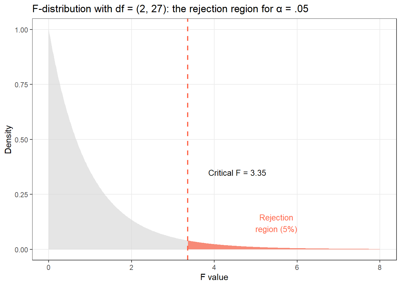
The larger the F-ratio, the more evidence against H₀. The significance of F is assessed against the F-distribution with degrees of freedom \((k-1, N-k)\).

Intuition for the F-ratio

Think of F as a signal-to-noise ratio. The numerator is the signal: how much do the group means differ? The denominator is the noise: how much do individuals within groups vary? A large F means the signal is much stronger than the noise — strong evidence that the groups differ.

If F = 1, the group differences are no larger than random variation within groups — no evidence of a real effect.

---

Exercises: The Logic of ANOVA

Q1. Why is it problematic to run multiple t-tests instead of ANOVA when comparing three or more groups?

t-tests cannot handle more than two groups, so they produce incorrect results
ANOVA is faster to compute, making it preferable for practical reasons
Each additional test inflates the family-wise Type I error rate, making false rejections increasingly likely
Multiple t-tests produce overly conservative results

---

Q2. An ANOVA returns F(3, 76) = 0.87. What does this suggest?

The ANOVA model is invalid and should be rerun
There is a significant difference between at least two groups
F < 1 always indicates a data entry error
The group means are not significantly different — the between-group variance is no larger than within-group noise

---

One-Way ANOVA

Section Overview

What you’ll learn: How to test whether three or more group means differ significantly; how to check assumptions; how to identify which groups differ using post-hoc tests

Key functions: aov(), summary(), TukeyHSD(), emmeans(), car::leveneTest()

Effect size: η² (eta-squared), ω² (omega-squared)

A one-way ANOVA tests whether the means of a numeric dependent variable differ across three or more levels of a single categorical independent variable (factor).

\[H_0: \mu_1 = \mu_2 = \cdots = \mu_k \quad \text{(all group means are equal)}\]
\[H_1: \text{At least one group mean differs from the others}\]

Assumptions

Before fitting a one-way ANOVA, the following assumptions should be verified:

Assumption	How to check
Independence of observations	Research design (each participant in one group only)
Normality of residuals within each group	Q-Q plots; Shapiro-Wilk test
Homogeneity of variances (homoskedasticity)	Levene’s test; boxplots
No extreme outliers	Boxplots; z-scores

ANOVA is relatively robust to mild violations of normality, especially with balanced designs (equal group sizes) and moderate-to-large sample sizes (n ≥ 15 per group). It is more sensitive to violations of homogeneity of variances, particularly with unequal group sizes.

Worked Example: Speech Rate Across Three Registers

Research question: Do speakers produce syllables at different rates in formal speech, informal conversation, and read-aloud tasks?

We simulate a dataset of syllables-per-second for 30 speakers (10 per register):

set.seed(42)  
n_per_group <- 10  
  
speech_rate <- data.frame(  
  Register    = rep(c("Formal", "Informal", "ReadAloud"), each = n_per_group),  
  SyllablesPS = c(  
    rnorm(n_per_group, mean = 4.2, sd = 0.6),   # Formal: slower  
    rnorm(n_per_group, mean = 5.4, sd = 0.7),   # Informal: fastest  
    rnorm(n_per_group, mean = 4.8, sd = 0.5)    # Read aloud: intermediate  
  )  
) |>  
  dplyr::mutate(Register = factor(Register,  
                                  levels = c("Formal", "ReadAloud", "Informal")))  

Step 1: Descriptive Statistics

Always start with a descriptive summary before running inferential tests:

speech_rate |>  
  dplyr::group_by(Register) |>  
  dplyr::summarise(  
    n    = n(),  
    M    = round(mean(SyllablesPS), 2),  
    SD   = round(sd(SyllablesPS), 2),  
    Mdn  = round(median(SyllablesPS), 2),  
    Min  = round(min(SyllablesPS), 2),  
    Max  = round(max(SyllablesPS), 2)  
  ) |>  
  flextable() |>  
  flextable::set_table_properties(width = .85, layout = "autofit") |>  
  flextable::theme_zebra() |>  
  flextable::fontsize(size = 12) |>  
  flextable::fontsize(size = 12, part = "header") |>  
  flextable::align_text_col(align = "center") |>  
  flextable::set_caption(caption = "Descriptive statistics: speech rate (syllables/second) by register.") |>  
  flextable::border_outer()  

Register	n	M	SD	Mdn	Min	Max
Formal	10	4.53	0.50	4.43	3.86	5.41
ReadAloud	10	4.71	0.58	4.66	3.91	5.75
Informal	10	5.29	1.14	5.26	3.54	7.00

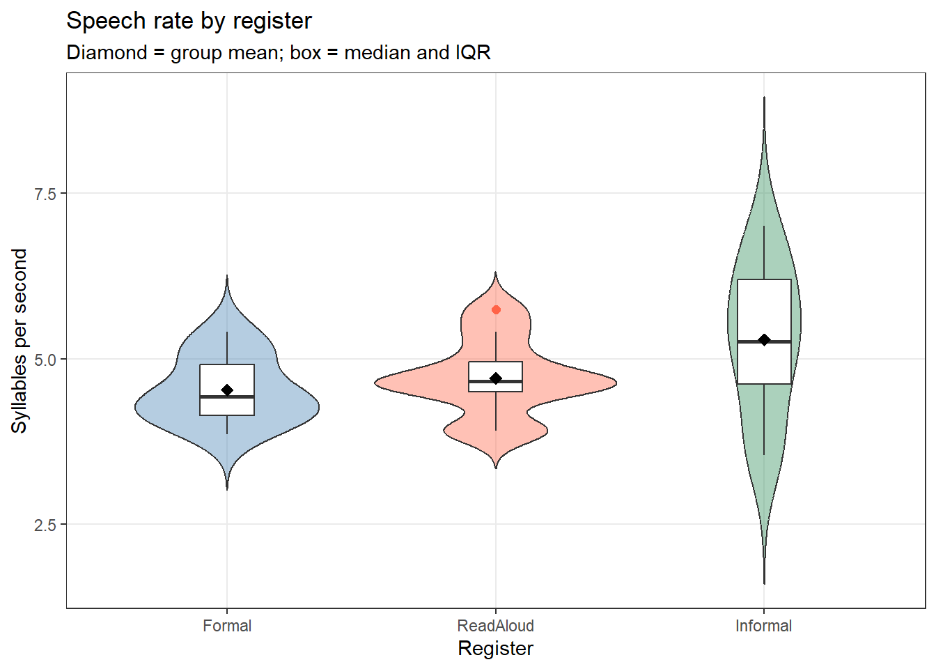
Step 2: Visualise the Data

ggplot(speech_rate, aes(x = Register, y = SyllablesPS, fill = Register)) +  
  geom_violin(alpha = 0.4, trim = FALSE) +  
  geom_boxplot(width = 0.2, fill = "white",  
               outlier.color = "tomato", outlier.size = 2) +  
  stat_summary(fun = mean, geom = "point",  
               shape = 18, size = 3, color = "black") +  
  scale_fill_manual(values = c("steelblue", "tomato", "seagreen")) +  
  theme_bw() +  
  theme(legend.position = "none", panel.grid.minor = element_blank()) +  
  labs(title = "Speech rate by register",  
       subtitle = "Diamond = group mean; box = median and IQR",  
       x = "Register", y = "Syllables per second")  

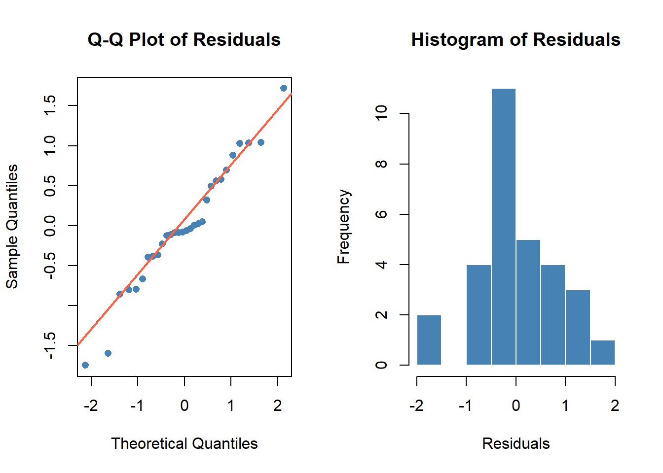
Step 3: Check Assumptions

Normality of residuals

Fit the model first, then inspect residuals:

anova_model <- aov(SyllablesPS ~ Register, data = speech_rate)  
  
# Q-Q plot of residuals  
par(mfrow = c(1, 2))  
qqnorm(residuals(anova_model), main = "Q-Q Plot of Residuals", pch = 16,  
       col = "steelblue")  
qqline(residuals(anova_model), col = "tomato", lwd = 2)  
  
hist(residuals(anova_model), breaks = 10, main = "Histogram of Residuals",  
     xlab = "Residuals", col = "steelblue", border = "white")  

par(mfrow = c(1, 1))  

# Shapiro-Wilk test on residuals  
shapiro.test(residuals(anova_model))  

    Shapiro-Wilk normality test

data:  residuals(anova_model)
W = 0.9699069501, p-value = 0.536631966

Homogeneity of variances (Levene’s test):

car::leveneTest(SyllablesPS ~ Register, data = speech_rate)  

Levene's Test for Homogeneity of Variance (center = median)
      Df F value  Pr(>F)  
group  2 3.22011 0.05569 .
      27                  
---
Signif. codes:  0 '***' 0.001 '**' 0.01 '*' 0.05 '.' 0.1 ' ' 1

What If Assumptions Are Violated?

• Non-normal residuals with sufficient sample size (n ≥ 15 per group): ANOVA is robust; proceed with caution and report the violation
  
• Non-normal residuals with small samples: use the Kruskal-Wallis test (non-parametric alternative)
  
• Unequal variances: use Welch’s ANOVA — oneway.test(y ~ group, var.equal = FALSE) — which does not assume homoskedasticity
  

Step 4: Fit and Interpret the ANOVA

summary(anova_model)  

            Df      Sum Sq     Mean Sq F value  Pr(>F)
Register     2  3.12293226 1.561466128 2.48088 0.10254
Residuals   27 16.99382771 0.629401026                

The ANOVA table shows:

• Df: degrees of freedom for the effect (k − 1 = 2) and error (N − k = 27)
  
• Sum Sq: sum of squares (SS) for each source of variance
  
• Mean Sq: mean square = Sum Sq / Df
  
• F value: the F-ratio = MS_between / MS_within
  
• Pr(>F): the p-value

Step 5: Effect Size

A significant F-ratio tells us that group means differ, but not how much they differ. We need an effect size.

Eta-squared (η²) is the proportion of total variance explained by the factor:

\[\eta^2 = \frac{SS_{\text{between}}}{SS_{\text{total}}}\]

Omega-squared (ω²) is a less biased alternative that corrects for the number of groups and sample size:

\[\omega^2 = \frac{SS_{\text{between}} - (k-1) \cdot MS_{\text{within}}}{SS_{\text{total}} + MS_{\text{within}}}\]

effectsize::eta_squared(anova_model, partial = FALSE)  

# Effect Size for ANOVA (Type I)

Parameter | Eta2 |       95% CI
-------------------------------
Register  | 0.16 | [0.00, 1.00]

- One-sided CIs: upper bound fixed at [1.00].

effectsize::omega_squared(anova_model, partial = FALSE)  

# Effect Size for ANOVA (Type I)

Parameter | Omega2 |       95% CI
---------------------------------
Register  |   0.09 | [0.00, 1.00]

- One-sided CIs: upper bound fixed at [1.00].

Statistic	Small	Medium	Large	Notes
η² (eta-squared)	.01	.06	.14	Biased upward; overestimates in small samples
ω² (omega-squared)	.01	.06	.14	Less biased; preferred for reporting

Step 6: Post-Hoc Tests

A significant one-way ANOVA tells us that at least one group mean differs — but not which pairs differ. Post-hoc tests perform all pairwise comparisons while controlling the family-wise error rate.

Choosing a Post-Hoc Test

Test	When to use
Tukey HSD	Equal or near-equal sample sizes; most common choice
Bonferroni	Conservative; best when you have few planned comparisons
Games-Howell	Unequal variances (heteroskedasticity)
Scheffé	Complex contrasts involving combinations of groups

For most linguistic research with balanced designs, Tukey HSD is the standard choice.

Tukey HSD via base R:

TukeyHSD(anova_model)  

  Tukey multiple comparisons of means
    95% family-wise confidence level

Fit: aov(formula = SyllablesPS ~ Register, data = speech_rate)

$Register
                             diff             lwr           upr          p adj
ReadAloud-Formal   0.182582172419 -0.697105318852 1.06226966369 0.864904394603
Informal-Formal    0.757202229708 -0.122485261563 1.63688972098 0.101712887808
Informal-ReadAloud 0.574620057289 -0.305067433982 1.45430754856 0.254862891479

Estimated marginal means and pairwise contrasts via emmeans (more flexible, works with complex designs):

emm <- emmeans::emmeans(anova_model, ~ Register)  
emm  

 Register  emmean    SE df lower.CL upper.CL
 Formal      4.53 0.251 27     4.01     5.04
 ReadAloud   4.71 0.251 27     4.20     5.23
 Informal    5.29 0.251 27     4.77     5.80

Confidence level used: 0.95 

# Pairwise contrasts with Tukey adjustment  
pairs(emm, adjust = "tukey")  

 contrast             estimate    SE df t.ratio p.value
 Formal - ReadAloud     -0.183 0.355 27  -0.515  0.8649
 Formal - Informal      -0.757 0.355 27  -2.134  0.1017
 ReadAloud - Informal   -0.575 0.355 27  -1.620  0.2549

P value adjustment: tukey method for comparing a family of 3 estimates 

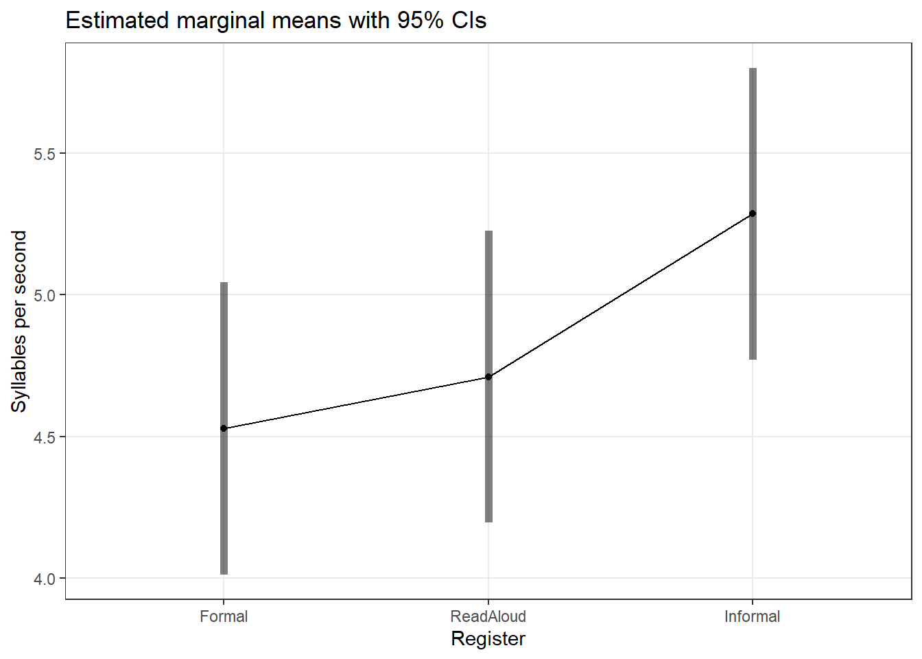
Visualise the pairwise comparisons:

emmeans::emmip(anova_model, ~ Register,  
               CIs = TRUE, style = "factor") +  
  theme_bw() +  
  theme(panel.grid.minor = element_blank()) +  
  labs(title = "Estimated marginal means with 95% CIs",  
       y = "Syllables per second", x = "Register")  

Reporting: One-Way ANOVA

A one-way ANOVA was conducted to examine whether speech rate (syllables per second) differed across three register types (Formal, Read Aloud, Informal). Levene’s test confirmed homogeneity of variances (p > .05), and residuals were approximately normal (Shapiro-Wilk: p > .05). The ANOVA revealed a significant main effect of Register (F(2, 27) = X.XX, p = .XXX, ω² = .XX). Post-hoc Tukey HSD comparisons showed that informal speech was significantly faster than formal speech (p = .XXX) and read-aloud speech (p = .XXX), while formal and read-aloud rates did not differ significantly (p = .XXX).

---

Exercises: One-Way ANOVA

Q1. A one-way ANOVA returns F(4, 95) = 2.87, p = .027. What can you conclude?

At least one pair of group means differs significantly; post-hoc tests are needed to identify which pairs
The effect is large because F > 1
The result is not significant because F < 3
All five groups differ significantly from each other

---

Q2. Levene’s test returns p = .003 for a one-way ANOVA with unequal group sizes. What should you do?

Remove the group with the highest variance
Use Welch's ANOVA (oneway.test(y ~ group, var.equal = FALSE)), which does not assume equal variances
Proceed with standard ANOVA — Levene's test is merely advisory
Switch to a paired t-test

---

Q3. Why is it important to report ω² rather than η² for ANOVA effect sizes in small samples?

They are equivalent — the choice is purely stylistic
η² is biased upward in small samples — it systematically overestimates the true population effect size; ω² corrects for this bias
η² cannot be computed when sample sizes are unequal
ω² is always larger than η², making effects look more impressive

---

Two-Way ANOVA

Section Overview

What you’ll learn: How to test the effects of two categorical factors simultaneously; what interaction effects are and how to interpret them; how to visualise factorial designs

Key concepts: Main effects, interaction effects, factorial design, interaction plot

Key functions: aov(), interaction.plot(), emmeans(), effectsize::eta_squared(partial = TRUE)

A two-way ANOVA (also called a factorial ANOVA) examines the effects of two categorical independent variables (factors) on a numeric dependent variable. It partitions variance into three components:

\[SS_{\text{total}} = SS_A + SS_B + SS_{A \times B} + SS_{\text{within}}\]

• Main effect of A: Does the dependent variable differ across levels of factor A, averaging across all levels of factor B?
  
• Main effect of B: Does the dependent variable differ across levels of factor B, averaging across all levels of factor A?
  
• Interaction effect A×B: Does the effect of factor A on the dependent variable depend on the level of factor B?

Interaction Effects Take Priority

Always examine the interaction term first. If the interaction is significant, the main effects cannot be interpreted independently — the effect of one factor depends on the level of the other. In this case, interpret the simple effects (the effect of factor A at each level of factor B) rather than main effects.

Worked Example: Vocabulary Score by Proficiency and Instruction Type

Research question: Do vocabulary test scores differ by learner proficiency level (Beginner, Advanced) and instruction type (Explicit, Implicit), and do these two factors interact?

set.seed(42)  
n <- 15   # per cell  
  
vocab_data <- data.frame(  
  Proficiency = rep(c("Beginner", "Advanced"), each = n * 2),  
  Instruction = rep(rep(c("Explicit", "Implicit"), each = n), 2),  
  Score = c(  
    # Beginners: explicit instruction helps a lot; implicit less so  
    rnorm(n, mean = 62, sd = 8),   # Beginner × Explicit  
    rnorm(n, mean = 48, sd = 9),   # Beginner × Implicit  
    # Advanced: explicit and implicit both work well  
    rnorm(n, mean = 78, sd = 7),   # Advanced × Explicit  
    rnorm(n, mean = 76, sd = 8)    # Advanced × Implicit  
  )  
) |>  
  dplyr::mutate(  
    Proficiency = factor(Proficiency, levels = c("Beginner", "Advanced")),  
    Instruction = factor(Instruction, levels = c("Explicit", "Implicit"))  
  )  

Descriptive Statistics

vocab_data |>  
  dplyr::group_by(Proficiency, Instruction) |>  
  dplyr::summarise(  
    n  = n(),  
    M  = round(mean(Score), 2),  
    SD = round(sd(Score), 2),  
    .groups = "drop"  
  ) |>  
  flextable() |>  
  flextable::set_table_properties(width = .75, layout = "autofit") |>  
  flextable::theme_zebra() |>  
  flextable::fontsize(size = 12) |>  
  flextable::fontsize(size = 12, part = "header") |>  
  flextable::align_text_col(align = "center") |>  
  flextable::set_caption(caption = "Vocabulary scores (M, SD) by proficiency and instruction type.") |>  
  flextable::border_outer()  

Proficiency	Instruction	n	M	SD
Beginner	Explicit	15	65.87	8.20
Beginner	Implicit	15	44.88	12.21
Advanced	Explicit	15	75.61	6.98
Advanced	Implicit	15	76.79	8.71

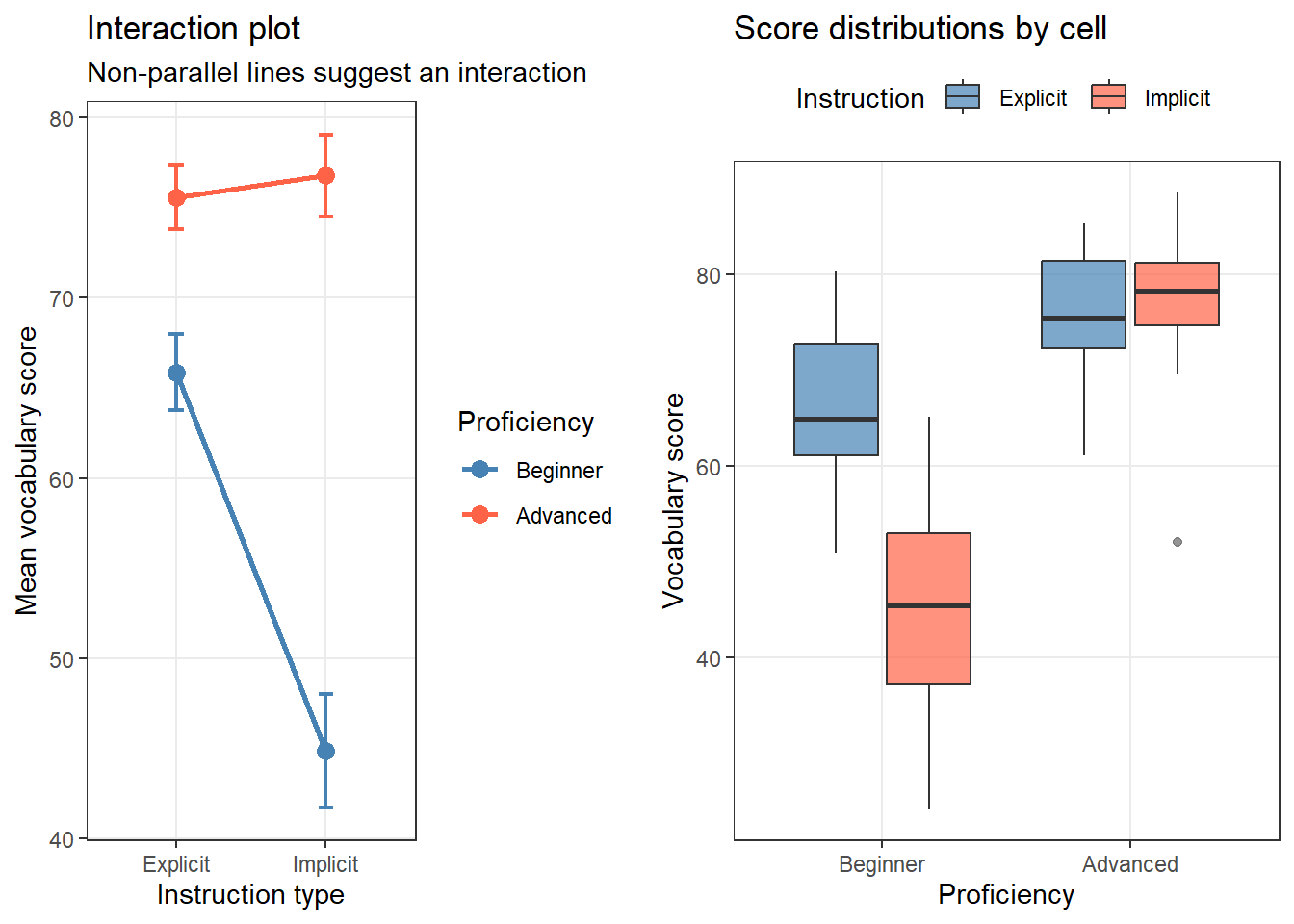
Visualise the Interaction

The interaction plot is the most informative visualisation for a factorial design. Parallel lines indicate no interaction; non-parallel (crossing or diverging) lines suggest an interaction.

# Summary for plotting  
twa_summary <- vocab_data |>  
  dplyr::group_by(Proficiency, Instruction) |>  
  dplyr::summarise(  
    M  = mean(Score),  
    SE = sd(Score) / sqrt(n()),  
    .groups = "drop"  
  )  
  
p1 <- ggplot(twa_summary,  
             aes(x = Instruction, y = M,  
                 color = Proficiency, group = Proficiency)) +  
  geom_line(linewidth = 1) +  
  geom_point(size = 3) +  
  geom_errorbar(aes(ymin = M - SE, ymax = M + SE),  
                width = 0.1, linewidth = 0.8) +  
  scale_color_manual(values = c("steelblue", "tomato")) +  
  theme_bw() +  
  theme(panel.grid.minor = element_blank()) +  
  labs(title = "Interaction plot",  
       subtitle = "Non-parallel lines suggest an interaction",  
       x = "Instruction type", y = "Mean vocabulary score",  
       color = "Proficiency")  
  
p2 <- ggplot(vocab_data,  
             aes(x = Proficiency, y = Score, fill = Instruction)) +  
  geom_boxplot(alpha = 0.7, outlier.color = "gray40") +  
  scale_fill_manual(values = c("steelblue", "tomato")) +  
  theme_bw() +  
  theme(panel.grid.minor = element_blank(), legend.position = "top") +  
  labs(title = "Score distributions by cell",  
       x = "Proficiency", y = "Vocabulary score", fill = "Instruction")  
  
cowplot::plot_grid(p1, p2, ncol = 2)  

The interaction plot shows that explicit instruction benefits beginners much more than implicit instruction, while advanced learners perform similarly under both conditions. This suggests an interaction.

Check Assumptions

twa_model <- aov(Score ~ Proficiency * Instruction, data = vocab_data)  
  
# Levene's test  
car::leveneTest(Score ~ Proficiency * Instruction, data = vocab_data)  

Levene's Test for Homogeneity of Variance (center = median)
      Df F value  Pr(>F)
group  3 1.12493 0.34682
      56                

# Normality of residuals  
shapiro.test(residuals(twa_model))  

    Shapiro-Wilk normality test

data:  residuals(twa_model)
W = 0.9832107045, p-value = 0.57811886

Fit the Two-Way ANOVA

summary(twa_model)  

                        Df     Sum Sq    Mean Sq  F value            Pr(>F)    
Proficiency              1 6502.45969 6502.45969 76.26482 0.000000000004886 ***
Instruction              1 1472.68022 1472.68022 17.27249        0.00011194 ***
Proficiency:Instruction  1 1844.45606 1844.45606 21.63291 0.000020592674808 ***
Residuals               56 4774.64878   85.26159                               
---
Signif. codes:  0 '***' 0.001 '**' 0.01 '*' 0.05 '.' 0.1 ' ' 1

Reading the Two-Way ANOVA Table

The output shows three rows of effects:

• Proficiency: main effect of proficiency level
  
• Instruction: main effect of instruction type
  
• Proficiency:Instruction: the interaction term

Because the interaction is significant, we focus on simple effects — the effect of Instruction within each level of Proficiency — rather than interpreting main effects in isolation.

Effect Sizes

For factorial designs, partial η² is reported instead of (total) η². Partial η² measures the proportion of variance explained by one effect after accounting for all other effects:

\[\eta^2_p = \frac{SS_{\text{effect}}}{SS_{\text{effect}} + SS_{\text{error}}}\]

effectsize::eta_squared(twa_model, partial = TRUE)  

# Effect Size for ANOVA (Type I)

Parameter               | Eta2 (partial) |       95% CI
-------------------------------------------------------
Proficiency             |           0.58 | [0.44, 1.00]
Instruction             |           0.24 | [0.09, 1.00]
Proficiency:Instruction |           0.28 | [0.13, 1.00]

- One-sided CIs: upper bound fixed at [1.00].

Simple Effects Analysis

When the interaction is significant, we decompose it by examining the effect of one factor at each level of the other:

emm_twa <- emmeans::emmeans(twa_model, ~ Instruction | Proficiency)  
emm_twa  

Proficiency = Beginner:
 Instruction emmean   SE df lower.CL upper.CL
 Explicit      65.9 2.38 56     61.1     70.6
 Implicit      44.9 2.38 56     40.1     49.7

Proficiency = Advanced:
 Instruction emmean   SE df lower.CL upper.CL
 Explicit      75.6 2.38 56     70.8     80.4
 Implicit      76.8 2.38 56     72.0     81.6

Confidence level used: 0.95 

# Simple effects: does instruction type matter within each proficiency group?  
pairs(emm_twa, adjust = "bonferroni")  

Proficiency = Beginner:
 contrast            estimate   SE df t.ratio p.value
 Explicit - Implicit    21.00 3.37 56   6.228  <.0001

Proficiency = Advanced:
 contrast            estimate   SE df t.ratio p.value
 Explicit - Implicit    -1.18 3.37 56  -0.350  0.7276

The simple effects analysis reveals that explicit instruction produces significantly higher scores than implicit instruction for beginners, but not for advanced learners — confirming the interaction.

Reporting: Two-Way ANOVA

A 2 × 2 factorial ANOVA examined the effects of proficiency level (Beginner, Advanced) and instruction type (Explicit, Implicit) on vocabulary scores. Levene’s test confirmed homogeneity of variances (F(3, 56) = X.XX, p > .05). There was a significant main effect of Proficiency (F(1, 56) = X.XX, p < .001, partial η² = .XX) and a significant Proficiency × Instruction interaction (F(1, 56) = X.XX, p = .XXX, partial η² = .XX). The main effect of Instruction was not significant (F(1, 56) = X.XX, p = .XXX). Simple effects analysis showed that explicit instruction produced significantly higher scores than implicit instruction for beginners (p < .001) but not for advanced learners (p = .XXX).

---

Exercises: Two-Way ANOVA

Q1. In a two-way ANOVA, the interaction term is significant. What should you do first?

Ignore the interaction and report only the main effects
Interpret the simple effects (the effect of one factor at each level of the other), not the main effects in isolation
Re-run the analysis as two separate one-way ANOVAs
Report the main effects first, then mention the interaction as secondary

---

Q2. An interaction plot shows two perfectly parallel lines. What does this indicate?

The data are normally distributed
A significant interaction — parallel lines always indicate interaction
The two factors have equal main effects
No interaction — the effect of one factor is the same at all levels of the other factor

---

Repeated Measures ANOVA

Section Overview

What you’ll learn: How to analyse designs where the same participants are measured across multiple conditions or time points; the sphericity assumption and its corrections

Key concepts: Within-subjects factor, sphericity, Mauchly’s test, Greenhouse-Geisser correction

Key functions: aov() with Error(), rstatix::anova_test(), emmeans()

A repeated measures ANOVA (also called a within-subjects ANOVA) is used when the same participants are measured under three or more conditions. Because measurements come from the same individuals, they are correlated — the repeated measures design removes between-subject variability, increasing statistical power.

The Sphericity Assumption

Repeated measures ANOVA requires an additional assumption not needed in independent ANOVA: sphericity. Sphericity requires that the variances of the differences between all pairs of conditions are equal.

Sphericity is tested using Mauchly’s test:
- p > .05: sphericity is not violated — proceed normally
- p ≤ .05: sphericity is violated — apply a correction to the degrees of freedom

The most common correction is the Greenhouse-Geisser correction (ε̂), which reduces the degrees of freedom to account for the violation. A more liberal alternative is the Huynh-Feldt correction. When sphericity is severely violated (ε̂ < .75), the Greenhouse-Geisser correction is preferred.

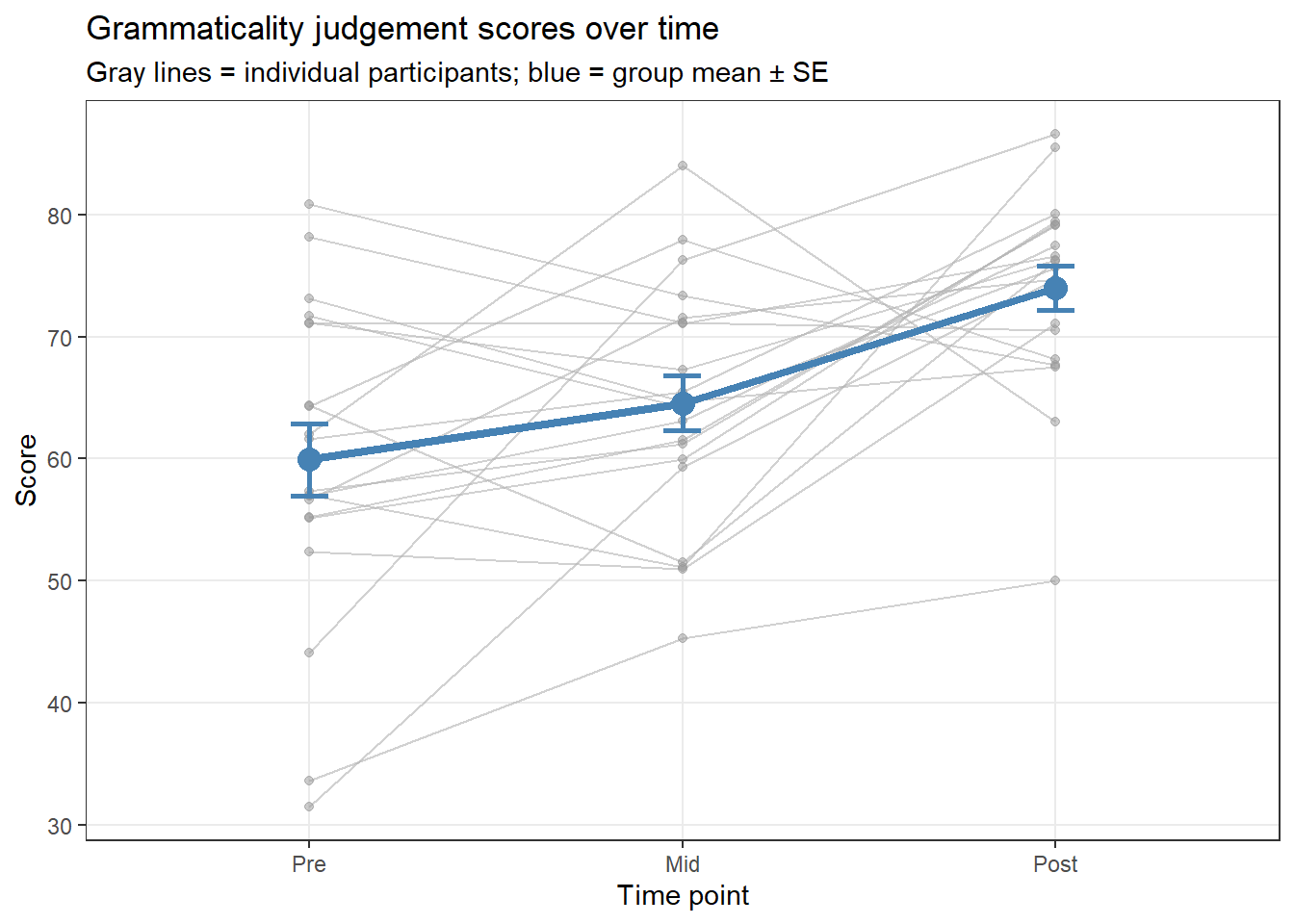
Worked Example: Grammaticality Judgements Across Three Time Points

Research question: Do grammaticality judgement scores change over three testing sessions (pre-instruction, mid-instruction, post-instruction)?

set.seed(42)  
n_participants <- 20  
  
rm_data <- data.frame(  
  Participant = factor(rep(1:n_participants, 3)),  
  Time        = factor(rep(c("Pre", "Mid", "Post"), each = n_participants),  
                       levels = c("Pre", "Mid", "Post")),  
  Score       = c(  
    rnorm(n_participants, mean = 58, sd = 10),   # Pre  
    rnorm(n_participants, mean = 67, sd = 9),    # Mid  
    rnorm(n_participants, mean = 74, sd = 8)     # Post  
  )  
)  

Descriptive Statistics and Visualisation

rm_data |>  
  dplyr::group_by(Time) |>  
  dplyr::summarise(  
    n  = n(),  
    M  = round(mean(Score), 2),  
    SD = round(sd(Score), 2),  
    .groups = "drop"  
  ) |>  
  flextable() |>  
  flextable::set_table_properties(width = .6, layout = "autofit") |>  
  flextable::theme_zebra() |>  
  flextable::fontsize(size = 12) |>  
  flextable::fontsize(size = 12, part = "header") |>  
  flextable::align_text_col(align = "center") |>  
  flextable::set_caption(caption = "Grammaticality judgement scores across three time points.") |>  
  flextable::border_outer()  

Time	n	M	SD
Pre	20	59.92	13.13
Mid	20	64.56	9.99
Post	20	73.99	8.19

# Individual trajectories + group mean  
rm_summary <- rm_data |>  
  dplyr::group_by(Time) |>  
  dplyr::summarise(M = mean(Score), SE = sd(Score)/sqrt(n()), .groups = "drop")  
  
ggplot(rm_data, aes(x = Time, y = Score, group = Participant)) +  
  geom_line(color = "gray70", alpha = 0.6, linewidth = 0.5) +  
  geom_point(color = "gray60", alpha = 0.5, size = 1.5) +  
  geom_line(data = rm_summary, aes(x = Time, y = M, group = 1),  
            color = "steelblue", linewidth = 1.5, inherit.aes = FALSE) +  
  geom_point(data = rm_summary, aes(x = Time, y = M),  
             color = "steelblue", size = 4, inherit.aes = FALSE) +  
  geom_errorbar(data = rm_summary,  
                aes(x = Time, ymin = M - SE, ymax = M + SE),  
                width = 0.1, color = "steelblue", linewidth = 1,  
                inherit.aes = FALSE) +  
  theme_bw() +  
  theme(panel.grid.minor = element_blank()) +  
  labs(title = "Grammaticality judgement scores over time",  
       subtitle = "Gray lines = individual participants; blue = group mean ± SE",  
       x = "Time point", y = "Score")  

Fit the Repeated Measures ANOVA

In base R, repeated measures ANOVA is specified using an Error() term:

rm_model <- aov(Score ~ Time + Error(Participant/Time), data = rm_data)  
summary(rm_model)  

Error: Participant
          Df     Sum Sq    Mean Sq F value Pr(>F)
Residuals 19 2973.10678 156.479304               

Error: Participant:Time
          Df     Sum Sq     Mean Sq  F value     Pr(>F)    
Time       2 2057.11086 1028.555429 11.26567 0.00014397 ***
Residuals 38 3469.39797   91.299946                        
---
Signif. codes:  0 '***' 0.001 '**' 0.01 '*' 0.05 '.' 0.1 ' ' 1

The rstatix package provides a more convenient interface that also performs Mauchly’s test and applies corrections automatically:

rm_data |>  
  rstatix::anova_test(  
    dv    = Score,  
    wid   = Participant,  
    within = Time  
  )  

ANOVA Table (type III tests)

$ANOVA
  Effect DFn DFd      F        p p<.05   ges
1   Time   2  38 11.266 0.000144     * 0.242

$`Mauchly's Test for Sphericity`
  Effect     W     p p<.05
1   Time 0.932 0.533      

$`Sphericity Corrections`
  Effect   GGe      DF[GG]    p[GG] p[GG]<.05   HFe      DF[HF]    p[HF]
1   Time 0.937 1.87, 35.59 0.000213         * 1.035 2.07, 39.35 0.000144
  p[HF]<.05
1         *

The output includes:
- F: the F-statistic
- p: the p-value (uncorrected)
- p<.05: significance indicator
- ges: generalised eta-squared (the recommended effect size for repeated measures designs)
- Mauchly’s W and p for the sphericity test
- GGe: the Greenhouse-Geisser epsilon (ε̂)
- p[GG]: the Greenhouse-Geisser corrected p-value

Post-Hoc Pairwise Comparisons

emm_rm <- emmeans::emmeans(rm_model, ~ Time)  
pairs(emm_rm, adjust = "bonferroni")  

 contrast   estimate   SE df t.ratio p.value
 Pre - Mid     -4.64 3.02 38  -1.536  0.3983
 Pre - Post   -14.07 3.02 38  -4.658  0.0001
 Mid - Post    -9.43 3.02 38  -3.121  0.0103

P value adjustment: bonferroni method for 3 tests 

Reporting: Repeated Measures ANOVA

A one-way repeated measures ANOVA examined whether grammaticality judgement scores changed across three time points (Pre, Mid, Post). Mauchly’s test indicated that [sphericity was/was not] violated (W = X.XX, p = .XXX). [If violated: The Greenhouse-Geisser correction was therefore applied (ε̂ = X.XX).] The ANOVA revealed a significant main effect of Time (F(X.XX, X.XX) = X.XX, p < .001, generalised η² = .XX). Bonferroni-corrected pairwise comparisons showed that scores increased significantly from Pre to Mid (p = .XXX) and from Mid to Post (p = .XXX).

---

Exercises: Repeated Measures ANOVA

Q1. What is the sphericity assumption in repeated measures ANOVA, and why does it matter?

Sphericity requires that all participants score equally across conditions
Sphericity requires that the variances of the differences between all pairs of conditions are equal; violations inflate the Type I error rate
Sphericity requires normal distribution of the dependent variable
Sphericity is another name for homogeneity of variances between groups

---

Q2. Mauchly’s test returns W = 0.71, p = .003 for a 4-level repeated measures factor. What should you report?

Switch to a between-subjects ANOVA since sphericity is violated
Report the uncorrected F-statistic — Mauchly's test is only advisory
Report the Huynh-Feldt correction, which is always preferred over Greenhouse-Geisser
Report the Greenhouse-Geisser corrected F-statistic and p-value, since sphericity is violated (p < .05)

---

MANOVA

Section Overview

What you’ll learn: When and why to use multiple dependent variables simultaneously; how MANOVA protects against inflated error rates across multiple outcomes; how to interpret multivariate test statistics and follow up with univariate ANOVAs

Key concepts: Multivariate test statistics (Pillai’s trace, Wilks’ λ, Hotelling’s T², Roy’s largest root); discriminant functions

Key functions: manova(), summary(), summary.aov()

MANOVA (Multivariate Analysis of Variance) extends ANOVA to designs with two or more dependent variables. Instead of testing group differences on each outcome separately (which would again inflate Type I error), MANOVA tests all outcomes simultaneously within a single multivariate framework.

When to Use MANOVA

Use MANOVA when:

• You have two or more correlated dependent variables measured on the same participants
  
• You want to understand whether groups differ across a profile of outcomes considered together
  
• You want to control the overall Type I error rate across multiple outcomes

Do not use MANOVA simply because you have multiple outcomes — if the outcomes are theoretically unrelated, separate ANOVAs with an appropriate correction (e.g., Bonferroni) may be more interpretable.

The Multivariate Test Statistics

MANOVA produces several test statistics, each with slightly different properties:

Statistic	Formula_logic	Robustness	Recommendation
Pillai's trace	Sum of explained variance in each discriminant dimension	Most robust; recommended when assumptions may be violated	Preferred for most applications
Wilks' λ	Product of (1 − explained variance) across dimensions	Traditional default; performs well when assumptions are met	Report alongside Pillai when assumptions met
Hotelling's trace	Sum of explained/unexplained variance ratios	Sensitive to non-normality	Rarely preferred
Roy's largest root	Variance on the first (largest) discriminant dimension only	Powerful but anti-conservative; only valid if one discriminant function dominates	Use with caution

Which Test Statistic to Report?

Pillai’s trace is the most robust to violations of multivariate normality and homogeneity of covariance matrices, and is the recommended default for most linguistic research. When the assumptions are well met and you have one dominant discriminant function, Wilks’ λ is a reasonable alternative.

Assumptions of MANOVA

MANOVA extends the ANOVA assumptions to the multivariate case:

Assumption	How to check
Multivariate normality	Q-Q plots per group per variable; Mardia’s test (rstatix::mshapiro_test())
Homogeneity of covariance matrices	Box’s M test (rstatix::box_m()) — note: very sensitive, treat cautiously
Independence of observations	Research design
No extreme multivariate outliers	Mahalanobis distance
No multicollinearity between DVs	Correlation matrix; if r > .90, consider combining or dropping variables

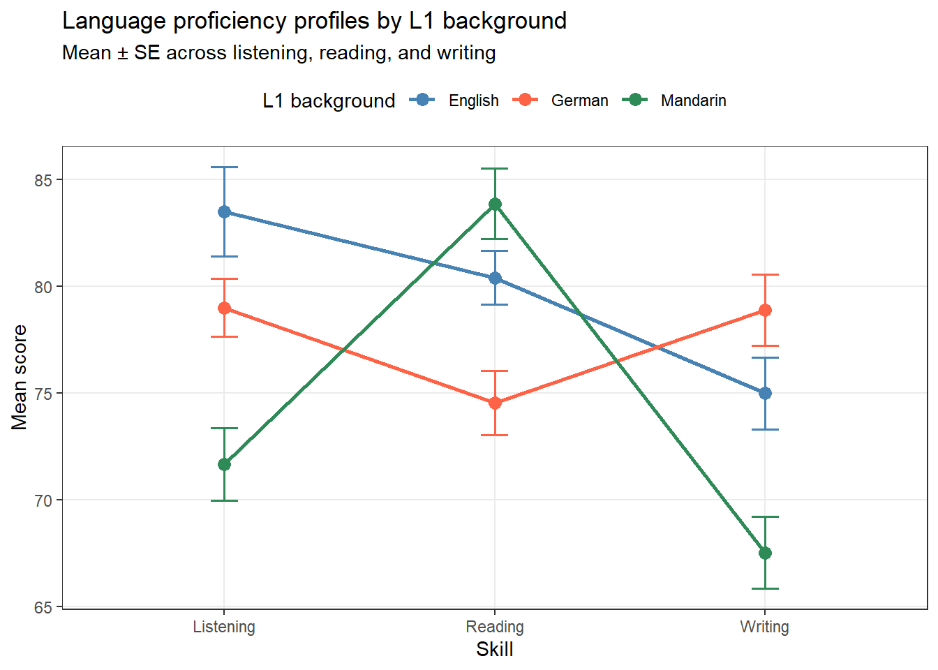
Worked Example: Language Proficiency Profiles Across Three L1 Backgrounds

Research question: Do speakers from three different L1 backgrounds (English, Mandarin, German) differ in their overall language proficiency profile, as measured by listening score, reading score, and writing score?

set.seed(42)  
n_per <- 25  
  
manova_data <- data.frame(  
  L1_Background = factor(rep(c("English", "Mandarin", "German"), each = n_per)),  
  Listening     = c(  
    rnorm(n_per, mean = 82, sd = 8),  
    rnorm(n_per, mean = 74, sd = 9),  
    rnorm(n_per, mean = 78, sd = 7)  
  ),  
  Reading = c(  
    rnorm(n_per, mean = 80, sd = 7),  
    rnorm(n_per, mean = 85, sd = 8),  
    rnorm(n_per, mean = 76, sd = 9)  
  ),  
  Writing = c(  
    rnorm(n_per, mean = 75, sd = 9),  
    rnorm(n_per, mean = 68, sd = 10),  
    rnorm(n_per, mean = 80, sd = 8)  
  )  
)  

Descriptive Statistics

manova_data |>  
  tidyr::pivot_longer(cols = c(Listening, Reading, Writing),  
                      names_to = "Skill", values_to = "Score") |>  
  dplyr::group_by(L1_Background, Skill) |>  
  dplyr::summarise(  
    M  = round(mean(Score), 1),  
    SD = round(sd(Score), 1),  
    .groups = "drop"  
  ) |>  
  tidyr::pivot_wider(names_from = Skill,  
                     values_from = c(M, SD)) |>  
  flextable() |>  
  flextable::set_table_properties(width = .99, layout = "autofit") |>  
  flextable::theme_zebra() |>  
  flextable::fontsize(size = 12) |>  
  flextable::fontsize(size = 12, part = "header") |>  
  flextable::align_text_col(align = "center") |>  
  flextable::set_caption(caption = "Proficiency scores (M, SD) by L1 background and skill.") |>  
  flextable::border_outer()  

L1_Background	M_Listening	M_Reading	M_Writing	SD_Listening	SD_Reading	SD_Writing
English	83.5	80.4	75.0	10.5	6.3	8.5
German	79.0	74.5	78.9	6.8	7.5	8.4
Mandarin	71.7	83.9	67.5	8.5	8.2	8.4

Visualise the Profiles

manova_data |>  
  tidyr::pivot_longer(cols = c(Listening, Reading, Writing),  
                      names_to = "Skill", values_to = "Score") |>  
  dplyr::group_by(L1_Background, Skill) |>  
  dplyr::summarise(M = mean(Score), SE = sd(Score)/sqrt(n()), .groups = "drop") |>  
  ggplot(aes(x = Skill, y = M,  
             color = L1_Background, group = L1_Background)) +  
  geom_line(linewidth = 1) +  
  geom_point(size = 3) +  
  geom_errorbar(aes(ymin = M - SE, ymax = M + SE),  
                width = 0.1, linewidth = 0.7) +  
  scale_color_manual(values = c("steelblue", "tomato", "seagreen")) +  
  theme_bw() +  
  theme(panel.grid.minor = element_blank(), legend.position = "top") +  
  labs(title = "Language proficiency profiles by L1 background",  
       subtitle = "Mean ± SE across listening, reading, and writing",  
       x = "Skill", y = "Mean score", color = "L1 background")  

The diverging profile lines suggest that the groups differ not just in overall proficiency but in their pattern of skill strengths — exactly the kind of question MANOVA is designed to answer.

Check Assumptions

# Multivariate normality per group (Shapiro-Wilk on each variable within each group)
manova_data |>
  tidyr::pivot_longer(cols = c(Listening, Reading, Writing),
                      names_to = "Skill", values_to = "Score") |>
  dplyr::group_by(L1_Background, Skill) |>
  dplyr::summarise(
    W = shapiro.test(Score)$statistic,
    p = shapiro.test(Score)$p.value,
    .groups = "drop"
  )

# A tibble: 9 × 4
  L1_Background Skill         W      p
  <fct>         <chr>     <dbl>  <dbl>
1 English       Listening 0.950 0.249 
2 English       Reading   0.945 0.193 
3 English       Writing   0.979 0.857 
4 German        Listening 0.907 0.0265
5 German        Reading   0.958 0.370 
6 German        Writing   0.957 0.351 
7 Mandarin      Listening 0.972 0.687 
8 Mandarin      Reading   0.920 0.0518
9 Mandarin      Writing   0.956 0.341 

# Homogeneity of covariance matrices (Box's M)
rstatix::box_m(
  data  = manova_data[, c("Listening", "Reading", "Writing")],
  group = manova_data$L1_Background
)

# A tibble: 1 × 4
  statistic p.value parameter method                                            
      <dbl>   <dbl>     <dbl> <chr>                                             
1      14.3   0.283        12 Box's M-test for Homogeneity of Covariance Matric…

# Correlation between DVs (check for multicollinearity)
cor(manova_data[, c("Listening", "Reading", "Writing")])

           Listening    Reading    Writing
Listening  1.0000000 -0.1440823  0.2903055
Reading   -0.1440823  1.0000000 -0.2745439
Writing    0.2903055 -0.2745439  1.0000000

Box’s M Test

Box’s M test is extremely sensitive — with moderate sample sizes it almost always rejects the null hypothesis of equal covariance matrices even when the violation is minor. Treat a significant Box’s M as a warning rather than an absolute contraindication. If Pillai’s trace is used as the test statistic, MANOVA remains robust to moderate violations.

Fit the MANOVA

# Bind outcome columns into a matrix (required by manova())  
outcome_matrix <- cbind(manova_data$Listening,  
                        manova_data$Reading,  
                        manova_data$Writing)  
  
manova_model <- manova(outcome_matrix ~ L1_Background, data = manova_data)  
  
# Pillai's trace (default and recommended)  
summary(manova_model, test = "Pillai")  

              Df  Pillai approx F num Df den Df    Pr(>F)    
L1_Background  2 0.54708   8.9115      6    142 2.962e-08 ***
Residuals     72                                             
---
Signif. codes:  0 '***' 0.001 '**' 0.01 '*' 0.05 '.' 0.1 ' ' 1

# Wilks' lambda for comparison  
summary(manova_model, test = "Wilks")  

              Df   Wilks approx F num Df den Df    Pr(>F)    
L1_Background  2 0.51243   9.2624      6    140 1.523e-08 ***
Residuals     72                                             
---
Signif. codes:  0 '***' 0.001 '**' 0.01 '*' 0.05 '.' 0.1 ' ' 1

Follow-Up Univariate ANOVAs

A significant MANOVA tells us the groups differ on the combination of outcomes. Follow-up univariate ANOVAs identify which individual outcomes drive the multivariate effect:

summary.aov(manova_model)  

 Response 1 :
              Df Sum Sq Mean Sq F value    Pr(>F)    
L1_Background  2 1782.7  891.37  11.725 3.909e-05 ***
Residuals     72 5473.7   76.02                      
---
Signif. codes:  0 '***' 0.001 '**' 0.01 '*' 0.05 '.' 0.1 ' ' 1

 Response 2 :
              Df Sum Sq Mean Sq F value    Pr(>F)    
L1_Background  2 1110.2  555.08  10.187 0.0001271 ***
Residuals     72 3923.3   54.49                      
---
Signif. codes:  0 '***' 0.001 '**' 0.01 '*' 0.05 '.' 0.1 ' ' 1

 Response 3 :
              Df Sum Sq Mean Sq F value    Pr(>F)    
L1_Background  2 1666.1  833.06  11.754 3.826e-05 ***
Residuals     72 5103.2   70.88                      
---
Signif. codes:  0 '***' 0.001 '**' 0.01 '*' 0.05 '.' 0.1 ' ' 1

For each significant univariate ANOVA, run post-hoc comparisons as you would for a standard one-way ANOVA:

# Post-hoc for Listening (if significant)  
listening_model <- aov(Listening ~ L1_Background, data = manova_data)  
TukeyHSD(listening_model)  

  Tukey multiple comparisons of means
    95% family-wise confidence level

Fit: aov(formula = Listening ~ L1_Background, data = manova_data)

$L1_Background
                       diff       lwr       upr     p adj
German-English    -4.501090 -10.40290  1.400720 0.1686844
Mandarin-English -11.830207 -17.73202 -5.928396 0.0000250
Mandarin-German   -7.329117 -13.23093 -1.427306 0.0110865

# Post-hoc for Reading  
reading_model <- aov(Reading ~ L1_Background, data = manova_data)  
TukeyHSD(reading_model)  

  Tukey multiple comparisons of means
    95% family-wise confidence level

Fit: aov(formula = Reading ~ L1_Background, data = manova_data)

$L1_Background
                      diff        lwr       upr     p adj
German-English   -5.861957 -10.858488 -0.865425 0.0174344
Mandarin-English  3.459438  -1.537094  8.455969 0.2288623
Mandarin-German   9.321394   4.324863 14.317926 0.0000856

# Post-hoc for Writing  
writing_model <- aov(Writing ~ L1_Background, data = manova_data)  
TukeyHSD(writing_model)  

  Tukey multiple comparisons of means
    95% family-wise confidence level

Fit: aov(formula = Writing ~ L1_Background, data = manova_data)

$L1_Background
                       diff        lwr       upr     p adj
German-English     3.906185  -1.792362  9.604732 0.2354814
Mandarin-English  -7.455601 -13.154148 -1.757053 0.0070242
Mandarin-German  -11.361786 -17.060333 -5.663238 0.0000275

Reporting: MANOVA

A one-way MANOVA examined whether L1 background (English, Mandarin, German) was associated with a profile of proficiency scores (Listening, Reading, Writing). Box’s M test [was/was not] significant (F(XX, XXXXX) = X.XX, p = .XXX), and Pillai’s trace was used as the test statistic. The MANOVA revealed a significant multivariate effect of L1 background (Pillai’s trace = X.XX, F(X, XX) = X.XX, p = .XXX). Univariate follow-up ANOVAs showed significant group differences for Listening (F(2, 72) = X.XX, p = .XXX, η² = .XX) and Writing (F(2, 72) = X.XX, p = .XXX, η² = .XX), but not for Reading (F(2, 72) = X.XX, p = .XXX).

---

Exercises: MANOVA

Q1. A researcher wants to compare three dialects of English on five phonetic measures simultaneously. Why is MANOVA preferable to five separate ANOVAs?

MANOVA tests all five outcomes simultaneously, keeping the family-wise Type I error rate at α = .05 and detecting multivariate group differences that might not be apparent in any individual ANOVA
MANOVA is faster to compute than five separate ANOVAs
MANOVA is required whenever you have more than three dependent variables
Separate ANOVAs would produce identical results to MANOVA

---

Q2. Why is Pillai’s trace generally recommended as the test statistic for MANOVA?

Pillai's trace always produces the largest F-statistic
Pillai's trace is the most robust to violations of multivariate normality and homogeneity of covariance matrices
Pillai's trace is less sensitive than Wilks' λ and therefore more conservative
Pillai's trace is the only statistic that adjusts for multiple dependent variables

---

ANCOVA

Section Overview

What you’ll learn: How to remove the influence of a continuous control variable (covariate) before testing group differences; how this increases statistical power and removes confounding; how to interpret adjusted means

Key concepts: Covariate, adjusted means, homogeneity of regression slopes

Key functions: aov() with covariate, emmeans() for adjusted means, car::Anova() for Type III SS

ANCOVA (Analysis of Covariance) combines ANOVA with linear regression. It tests whether group means on a dependent variable differ after controlling for one or more continuous covariates. ANCOVA serves two related purposes:

1. Reducing error variance: By explaining some of the within-group variability via the covariate, ANCOVA increases statistical power
   
2. Removing confounding: If groups differ on a variable that also predicts the outcome (a confound), ANCOVA statistically equates the groups on that variable before testing the group effect

Key Assumptions of ANCOVA

ANCOVA requires all ANOVA assumptions plus two additional ones:

Assumption	Description	How to check
Linear relationship between covariate and DV	The covariate should correlate linearly with the outcome	Scatterplot; correlation
Homogeneity of regression slopes	The relationship between covariate and DV must be the same in all groups (no group × covariate interaction)	Test the interaction term: aov(DV ~ group * covariate)
Independence of covariate and group factor	The covariate should not itself be affected by the group manipulation (especially in experiments)	Design consideration

The Homogeneity of Regression Slopes Assumption

If the slopes relating the covariate to the outcome differ across groups, the covariate adjusts scores differently in different groups — making the adjusted means uninterpretable. Always test this assumption by including the group × covariate interaction in the model. If the interaction is significant, ANCOVA assumptions are violated and a different approach (e.g., moderated regression) is needed.

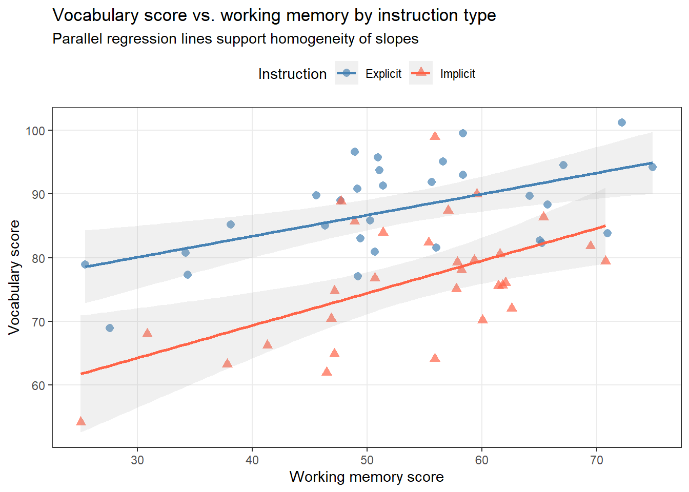
Worked Example: Vocabulary Scores Controlling for Working Memory

Research question: Does instruction type (Explicit vs. Implicit) affect vocabulary test scores, after controlling for working memory capacity?

Rationale: Groups may differ in working memory, which independently predicts vocabulary learning. ANCOVA removes this confound, revealing whether instruction type has an effect beyond what working memory alone would predict.

set.seed(42)  
n <- 30  # per group  
  
ancova_data <- data.frame(  
  Instruction    = factor(rep(c("Explicit", "Implicit"), each = n)),  
  WorkingMemory  = c(rnorm(n, mean = 52, sd = 10),  
                     rnorm(n, mean = 55, sd = 10)),  # slightly higher in Implicit group  
  VocabScore     = NA  
)  
  
# Vocabulary is affected by both instruction and working memory  
ancova_data$VocabScore <- with(ancova_data,  
  ifelse(Instruction == "Explicit", 65, 55) +    # instruction effect  
  0.4 * WorkingMemory +                           # working memory effect  
  rnorm(nrow(ancova_data), 0, 8)                  # noise  
)  

Step 1: Check That Covariate Predicts the Outcome

ggplot(ancova_data, aes(x = WorkingMemory, y = VocabScore,  
                         color = Instruction, shape = Instruction)) +  
  geom_point(alpha = 0.7, size = 2.5) +  
  geom_smooth(method = "lm", se = TRUE, alpha = 0.15) +  
  scale_color_manual(values = c("steelblue", "tomato")) +  
  theme_bw() +  
  theme(panel.grid.minor = element_blank(), legend.position = "top") +  
  labs(title = "Vocabulary score vs. working memory by instruction type",  
       subtitle = "Parallel regression lines support homogeneity of slopes",  
       x = "Working memory score", y = "Vocabulary score",  
       color = "Instruction", shape = "Instruction")  

Approximately parallel lines suggest that the relationship between working memory and vocabulary is similar across groups — supporting the homogeneity of slopes assumption.

Step 2: Test Homogeneity of Regression Slopes

# Include the interaction to test homogeneity of slopes  
slopes_test <- aov(VocabScore ~ Instruction * WorkingMemory, data = ancova_data)  
car::Anova(slopes_test, type = "III")  

Anova Table (Type III tests)

Response: VocabScore
                          Sum Sq Df  F value    Pr(>F)    
(Intercept)               7673.3  1 140.8085 < 2.2e-16 ***
Instruction                284.6  1   5.2218  0.026114 *  
WorkingMemory              502.0  1   9.2124  0.003643 ** 
Instruction:WorkingMemory   59.9  1   1.0985  0.299090    
Residuals                 3051.7 56                       
---
Signif. codes:  0 '***' 0.001 '**' 0.01 '*' 0.05 '.' 0.1 ' ' 1

A non-significant interaction (p > .05) confirms that the slopes are homogeneous — ANCOVA is appropriate.

Step 3: Fit the ANCOVA

With the assumption verified, we fit the ANCOVA (covariate enters first to ensure it is controlled for):

ancova_model <- aov(VocabScore ~ WorkingMemory + Instruction, data = ancova_data)  
car::Anova(ancova_model, type = "III")  

Anova Table (Type III tests)

Response: VocabScore
               Sum Sq Df F value    Pr(>F)    
(Intercept)   11235.8  1 205.826 < 2.2e-16 ***
WorkingMemory  1273.6  1  23.331 1.065e-05 ***
Instruction    2042.4  1  37.415 9.254e-08 ***
Residuals      3111.6 57                      
---
Signif. codes:  0 '***' 0.001 '**' 0.01 '*' 0.05 '.' 0.1 ' ' 1

Type I vs. Type III Sums of Squares

• Type I SS (sequential): Each effect is adjusted only for effects that appear earlier in the model formula. Order matters — use only with orthogonal (balanced, uncorrelated) designs.
  
• Type III SS (partial): Each effect is adjusted for all other effects simultaneously. Order does not matter — use with ANCOVA and unbalanced designs.

Always use car::Anova(model, type = "III") for ANCOVA to ensure correct Type III SS.

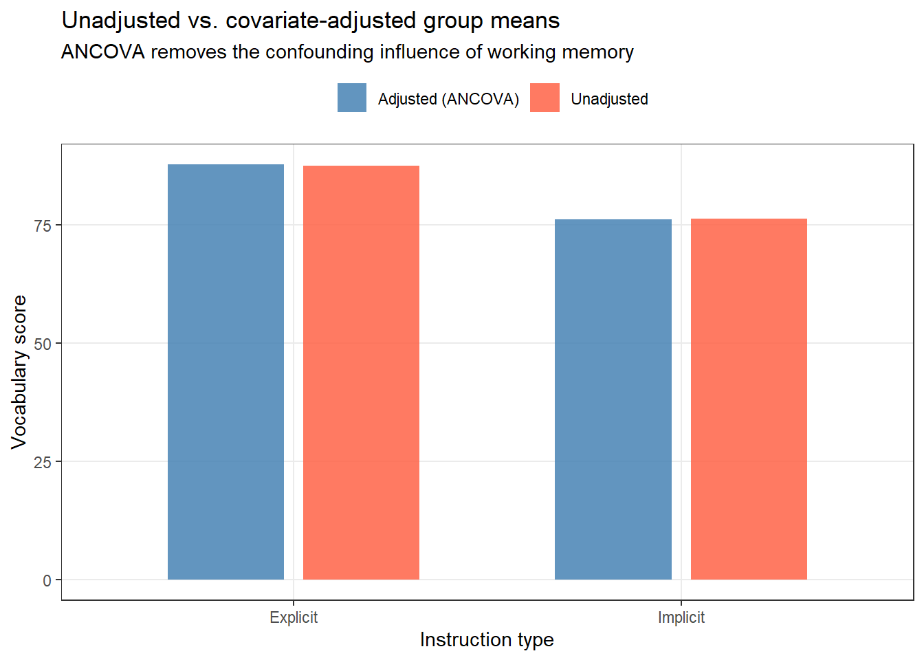
Step 4: Adjusted Means

The most important output from ANCOVA is the adjusted means — the estimated group means after statistically controlling for the covariate. These represent what the group means would be if all groups had the same covariate value (typically the grand mean).

# Estimated marginal means (adjusted for working memory)  
emm_ancova <- emmeans::emmeans(ancova_model, ~ Instruction)  
emm_ancova  

 Instruction emmean   SE df lower.CL upper.CL
 Explicit      87.8 1.35 57     85.1     90.5
 Implicit      76.1 1.35 57     73.4     78.8

Confidence level used: 0.95 

# Pairwise comparison of adjusted means  
pairs(emm_ancova)  

 contrast            estimate   SE df t.ratio p.value
 Explicit - Implicit     11.7 1.91 57   6.117  <.0001

# Compare unadjusted vs. adjusted means  
raw_means <- ancova_data |>  
  dplyr::group_by(Instruction) |>  
  dplyr::summarise(Mean = mean(VocabScore), Type = "Unadjusted", .groups = "drop")  
  
adj_means <- as.data.frame(emm_ancova) |>  
  dplyr::select(Instruction, emmean) |>  
  dplyr::rename(Mean = emmean) |>  
  dplyr::mutate(Type = "Adjusted (ANCOVA)")  
  
combined_means <- dplyr::bind_rows(raw_means, adj_means)  
  
ggplot(combined_means, aes(x = Instruction, y = Mean,  
                            fill = Type, group = Type)) +  
  geom_col(position = position_dodge(0.7), width = 0.6, alpha = 0.85) +  
  scale_fill_manual(values = c("steelblue", "tomato")) +  
  theme_bw() +  
  theme(panel.grid.minor = element_blank(), legend.position = "top") +  
  labs(title = "Unadjusted vs. covariate-adjusted group means",  
       subtitle = "ANCOVA removes the confounding influence of working memory",  
       x = "Instruction type", y = "Vocabulary score", fill = "")  

Step 5: Effect Size

effectsize::eta_squared(ancova_model, partial = TRUE)  

# Effect Size for ANOVA (Type I)

Parameter     | Eta2 (partial) |       95% CI
---------------------------------------------
WorkingMemory |           0.27 | [0.12, 1.00]
Instruction   |           0.40 | [0.24, 1.00]

- One-sided CIs: upper bound fixed at [1.00].

Reporting: ANCOVA

An ANCOVA was conducted to examine whether instruction type (Explicit vs. Implicit) affected vocabulary scores, after controlling for working memory capacity. The homogeneity of regression slopes assumption was verified — the interaction between instruction type and working memory was not significant (F(1, 56) = X.XX, p = .XXX). Working memory was a significant covariate (F(1, 57) = X.XX, p < .001, partial η² = .XX). After controlling for working memory, there was a significant main effect of instruction type (F(1, 57) = X.XX, p = .XXX, partial η² = .XX). Adjusted means indicated that explicit instruction (M_adj = XX.X) produced higher scores than implicit instruction (M_adj = XX.X).

---

Exercises: ANCOVA

Q1. What are the two main purposes of including a covariate in ANCOVA?

Replacing a missing second independent variable and simplifying the model
Reducing residual error variance (increasing power) and statistically removing the confounding influence of the covariate on the group comparison
Increasing the sample size and reducing the number of groups
Making the dependent variable normally distributed and removing outliers

---

Q2. The homogeneity of regression slopes test returns F(1, 56) = 7.23, p = .009. What does this mean for your ANCOVA?

Switch to MANOVA, which does not require homogeneous slopes
Remove the covariate from the model and run a standard ANOVA
ANCOVA is not appropriate — the covariate has a different relationship with the outcome in different groups; consider moderated regression instead
ANCOVA is still appropriate — this test only affects the covariate's significance

---

Q3. What is the difference between unadjusted means and adjusted means in ANCOVA?

Adjusted means are estimated group means after statistically controlling for the covariate — they represent what the means would be if all groups had the same covariate value
Adjusted means are means after removing outliers from the dataset
Adjusted means are standardised (z-score) versions of the raw means
Adjusted means include a Bonferroni correction for multiple comparisons

---

Effect Sizes and Statistical Power

Section Overview

What you’ll learn: How to quantify the practical importance of ANOVA results; the difference between η², partial η², ω², and Cohen’s f; a brief introduction to power analysis for ANOVA designs

Statistical significance tells us whether an effect exists; effect sizes tell us how large it is. Always report effect sizes alongside F-statistics and p-values.

Summary of Effect Size Measures for ANOVA

Measure	Formula	Small	Medium	Large	When to use
η² (eta-squared)	SS_effect / SS_total	.01	.06	.14	One-way ANOVA; total variance is meaningful
partial η²	SS_effect / (SS_effect + SS_error)	.01	.06	.14	Factorial ANOVA/ANCOVA; each effect assessed against error only
ω² (omega-squared)	Bias-corrected η²	.01	.06	.14	One-way ANOVA; preferred for small samples (less biased)
partial ω²	Bias-corrected partial η²	.01	.06	.14	Factorial ANOVA/ANCOVA; less biased than partial η²
Cohen's f	√(η² / (1 − η²))	.10	.25	.40	Power analysis; Cohen's conventions

Computing Effect Sizes in R

# Using the one-way ANOVA model from earlier  
anova_model <- aov(SyllablesPS ~ Register, data = speech_rate)  
  
# eta-squared (total)  
effectsize::eta_squared(anova_model, partial = FALSE)  

# Effect Size for ANOVA (Type I)

Parameter | Eta2 |       95% CI
-------------------------------
Register  | 0.16 | [0.00, 1.00]

- One-sided CIs: upper bound fixed at [1.00].

# partial eta-squared  
effectsize::eta_squared(anova_model, partial = TRUE)  

# Effect Size for ANOVA

Parameter | Eta2 |       95% CI
-------------------------------
Register  | 0.16 | [0.00, 1.00]

- One-sided CIs: upper bound fixed at [1.00].

# omega-squared (less biased; preferred for small samples)  
effectsize::omega_squared(anova_model, partial = FALSE)  

# Effect Size for ANOVA (Type I)

Parameter | Omega2 |       95% CI
---------------------------------
Register  |   0.09 | [0.00, 1.00]

- One-sided CIs: upper bound fixed at [1.00].

# Cohen's f (for power analysis)  
effectsize::cohens_f(anova_model)  

# Effect Size for ANOVA

Parameter | Cohen's f |      95% CI
-----------------------------------
Register  |      0.43 | [0.00, Inf]

- One-sided CIs: upper bound fixed at [Inf].

A Brief Note on Power Analysis

Statistical power is the probability of correctly detecting a true effect (i.e., rejecting H₀ when H₁ is true). The conventional target is power ≥ .80. Power depends on:

• Effect size (larger effects are easier to detect)
  
• Sample size (more participants → more power)
  
• Significance level α (stricter α → less power)
  
• Number of groups (more groups → more df needed)

The pwr package performs power analysis for ANOVA:

# install.packages("pwr")  
library(pwr)  
  
# What sample size is needed per group for:  
# - 3 groups (k = 3)  
# - medium effect (f = 0.25)  
# - α = .05, power = .80?  
pwr::pwr.anova.test(  
  k     = 3,       # number of groups  
  f     = 0.25,    # Cohen's f (medium effect)  
  sig.level = 0.05,  
  power = 0.80  
)  

     Balanced one-way analysis of variance power calculation 

              k = 3
              n = 52.3966
              f = 0.25
      sig.level = 0.05
          power = 0.8

NOTE: n is number in each group

This tells us the required sample size per group to achieve 80% power with a medium effect and three groups.

---

Reporting Standards

Clear, complete reporting allows readers to evaluate and reproduce your analyses. This section provides the key conventions and model reporting paragraphs.

APA-Style Conventions

Reporting Checklist for ANOVA-Family Tests

For every analysis, report:

• F-statistic with degrees of freedom: F(df_between, df_within) = X.XX
  
• p-value (exact where possible; p < .001 when very small)
  
• Effect size with confidence interval: partial η² = .XX, 95% CI [.XX, .XX]
  
• Group means and SDs (or a summary table)
  
• Assumption checks: Levene’s test, Shapiro-Wilk (or Q-Q plot description)
  
• Post-hoc tests: method used, adjusted p-values for each comparison
  
• For ANCOVA: adjusted means and the covariate F-statistic
  
• For repeated measures: Mauchly’s W, ε̂ if corrected, corrected df
  

Quick Reference: Test Selection

Research design	Test	R function	Effect size
3+ independent groups, 1 DV	One-way ANOVA	aov(y ~ group)	ω² or η²
3+ independent groups, 1 DV, unequal variances	Welch's ANOVA	oneway.test(y ~ group, var.equal = FALSE)	η²
3+ independent groups, 1 DV, non-normal data	Kruskal-Wallis test	kruskal.test(y ~ group)	ε² (rank-based)
2 factors (independent groups), 1 DV	Two-way (factorial) ANOVA	aov(y ~ A * B)	partial η² per effect
Same participants across 3+ conditions	Repeated measures ANOVA	aov(y ~ time + Error(id/time))	Generalised η²
Same participants across 3+ conditions, non-normal	Friedman test	friedman.test(y ~ time | id)	Kendall's W
3+ groups, 2+ DVs simultaneously	MANOVA	manova(cbind(y1,y2) ~ group)	Pillai's trace; univariate partial η²
3+ groups, 1 DV, controlling for a continuous variable	ANCOVA	aov(y ~ covariate + group)	partial η² (adjusted)

Model Reporting Paragraphs

One-way ANOVA

A one-way ANOVA examined whether speech rate (syllables per second) differed across three register types (Formal, Read Aloud, Informal). Levene’s test confirmed homogeneity of variances (F(2, 27) = X.XX, p = .XXX), and Shapiro-Wilk tests on residuals within each group indicated approximately normal distributions (all p > .05). The ANOVA revealed a significant main effect of Register (F(2, 27) = X.XX, p = .XXX, ω² = .XX, 95% CI [.XX, .XX]). Tukey HSD post-hoc comparisons showed that informal speech (M = 5.41, SD = 0.70) was significantly faster than both formal speech (M = 4.19, SD = 0.60; p < .001) and read-aloud speech (M = 4.80, SD = 0.50; p = .XXX).

Two-way ANOVA with significant interaction

A 2 × 2 factorial ANOVA examined the effects of Proficiency (Beginner, Advanced) and Instruction type (Explicit, Implicit) on vocabulary scores. The interaction between Proficiency and Instruction type was significant (F(1, 56) = X.XX, p = .XXX, partial η² = .XX), indicating that the effect of instruction type depended on learner proficiency. Simple effects analysis showed that explicit instruction produced significantly higher scores than implicit instruction for beginners (p < .001; M_diff = X.XX) but not for advanced learners (p = .XXX; M_diff = X.XX).

ANCOVA

An ANCOVA was conducted to examine whether instruction type (Explicit vs. Implicit) affected vocabulary test scores after controlling for working memory capacity. The homogeneity of regression slopes assumption was met — the Instruction × Working Memory interaction was non-significant (F(1, 56) = X.XX, p = .XXX). Working memory was a significant covariate (F(1, 57) = X.XX, p < .001, partial η² = .XX). After adjusting for working memory, instruction type had a significant effect on vocabulary scores (F(1, 57) = X.XX, p = .XXX, partial η² = .XX). Adjusted means showed higher scores for explicit (M_adj = XX.X, SE = X.X) than implicit instruction (M_adj = XX.X, SE = X.X).

MANOVA

A one-way MANOVA examined whether L1 background (English, Mandarin, German) was associated with a proficiency profile comprising Listening, Reading, and Writing scores (n = 75; 25 per group). Pillai’s trace was used as the test statistic given its robustness to assumption violations. The MANOVA revealed a significant multivariate effect of L1 background (Pillai’s trace = X.XX, F(X, XX) = X.XX, p = .XXX). Univariate follow-up ANOVAs with Bonferroni correction (α_adjusted = .017) showed significant group differences for Listening (F(2, 72) = X.XX, p = .XXX, η² = .XX) and Writing (F(2, 72) = X.XX, p = .XXX, η² = .XX) but not Reading (F(2, 72) = X.XX, p = .XXX).

---

Citation & Session Info

Citation

Martin Schweinberger. 2026. ANOVA, MANOVA, and ANCOVA using R. The Language Technology and Data Analysis Laboratory (LADAL), The University of Queensland, Australia. url: https://ladal.edu.au/tutorials/anova/anova.html (Version 2026.03.27), doi: 10.5281/zenodo.19242479.

@manual{martinschweinberger2026anova,
  author       = {Martin Schweinberger},
  title        = {ANOVA, MANOVA, and ANCOVA using R},
  year         = {2026},
  note         = {https://ladal.edu.au/tutorials/anova/anova.html},
  organization = {The Language Technology and Data Analysis Laboratory (LADAL), The University of Queensland, Australia},
  edition      = {2026.03.27}
  doi      = {10.5281/zenodo.19242479}
}

sessionInfo()  

R version 4.4.2 (2024-10-31 ucrt)
Platform: x86_64-w64-mingw32/x64
Running under: Windows 11 x64 (build 26200)

Matrix products: default


locale:
[1] LC_COLLATE=English_United States.utf8 
[2] LC_CTYPE=English_United States.utf8   
[3] LC_MONETARY=English_United States.utf8
[4] LC_NUMERIC=C                          
[5] LC_TIME=English_United States.utf8    

time zone: Australia/Brisbane
tzcode source: internal

attached base packages:
[1] stats     graphics  grDevices datasets  utils     methods   base     

other attached packages:
 [1] pwr_1.3-0        psych_2.4.12     cowplot_1.2.0    broom_1.0.7     
 [5] rstatix_0.7.2    ggpubr_0.6.0     car_3.1-3        carData_3.0-5   
 [9] emmeans_1.10.7   report_0.6.3     effectsize_1.0.1 flextable_0.9.7 
[13] tidyr_1.3.2      ggplot2_4.0.2    dplyr_1.2.0      checkdown_0.0.13

loaded via a namespace (and not attached):
 [1] tidyselect_1.2.1        farver_2.1.2            S7_0.2.1               
 [4] fastmap_1.2.0           TH.data_1.1-3           fontquiver_0.2.1       
 [7] bayestestR_0.17.0       digest_0.6.39           estimability_1.5.1     
[10] lifecycle_1.0.5         survival_3.7-0          magrittr_2.0.3         
[13] compiler_4.4.2          rlang_1.1.7             tools_4.4.2            
[16] utf8_1.2.4              yaml_2.3.10             data.table_1.17.0      
[19] knitr_1.51              ggsignif_0.6.4          labeling_0.4.3         
[22] askpass_1.2.1           htmlwidgets_1.6.4       mnormt_2.1.1           
[25] xml2_1.3.6              RColorBrewer_1.1-3      multcomp_1.4-28        
[28] abind_1.4-8             withr_3.0.2             purrr_1.0.4            
[31] grid_4.4.2              datawizard_1.3.0        gdtools_0.4.1          
[34] xtable_1.8-4            scales_1.4.0            MASS_7.3-61            
[37] insight_1.4.6           cli_3.6.4               mvtnorm_1.3-3          
[40] rmarkdown_2.30          ragg_1.3.3              generics_0.1.3         
[43] rstudioapi_0.17.1       commonmark_2.0.0        parameters_0.28.3      
[46] splines_4.4.2           parallel_4.4.2          vctrs_0.7.1            
[49] Matrix_1.7-2            sandwich_3.1-1          jsonlite_1.9.0         
[52] fontBitstreamVera_0.1.1 litedown_0.9            Formula_1.2-5          
[55] systemfonts_1.2.1       glue_1.8.0              codetools_0.2-20       
[58] gtable_0.3.6            tibble_3.2.1            pillar_1.10.1          
[61] htmltools_0.5.9         openssl_2.3.2           R6_2.6.1               
[64] textshaping_1.0.0       evaluate_1.0.3          lattice_0.22-6         
[67] markdown_2.0            backports_1.5.0         renv_1.1.1             
[70] fontLiberation_0.1.0    Rcpp_1.0.14             zip_2.3.2              
[73] uuid_1.2-1              nlme_3.1-166            coda_0.19-4.1          
[76] mgcv_1.9-1              officer_0.6.7           xfun_0.56              
[79] zoo_1.8-13              pkgconfig_2.0.3        

AI Transparency Statement

This tutorial was revised and substantially expanded with the assistance of Claude (claude.ai), a large language model created by Anthropic. Claude was used to restructure the document into Quarto format, expand the theoretical introduction, add the new sections and accompanying callouts, expand interpretation guidance across all sections, write the new quiz questions and detailed answer explanations, and produce the comparison summary table. All content was reviewed, edited, and approved by the author (Martin Schweinberger), who takes full responsibility for its accuracy.

Back to top

Back to HOME

References