Processing and Analysing Eye-Tracking Data in R

Introduction

Eye-tracking is one of the most powerful methods available to researchers studying real-time language processing. By recording where participants look — and when — as they hear or read linguistic input, eye-tracking provides millisecond-resolution evidence about how the mind constructs meaning, retrieves words, and resolves structural ambiguities. The technique rests on a simple but powerful insight: eye movements are tightly time-locked to ongoing cognitive processing (Tanenhaus et al. 1995; Allopenna, Magnuson, and Tanenhaus 1998). When a listener hears a spoken word, their eyes move to a picture of the named object within approximately 200 ms — faster than they can consciously plan a deliberate response. This tight coupling between language and gaze makes eye movements a privileged window into the real-time workings of the language system.

The Visual World Paradigm (VWP) in particular has become a cornerstone of psycholinguistic research. In the canonical version of the paradigm, introduced by Tanenhaus et al. (1995), participants listen to spoken sentences while viewing a display of objects or images, and the time course of their eye movements to those images reflects the unfolding of language comprehension in real time. Since that foundational study, the VWP has been used to investigate an extraordinary range of phenomena: spoken word recognition and lexical competition (Allopenna, Magnuson, and Tanenhaus 1998), the use of grammatical gender in word recognition (Dahan et al. 2000), syntactic ambiguity resolution, referential processing, predictive language use, and many more. The paradigm has proven especially valuable because it captures the time course of processing — not just whether listeners are successful, but when and how quickly they arrive at an interpretation.

Despite its power, eye-tracking data is notoriously complex to work with. Raw data files contain thousands of gaze samples per participant, spread across multiple trials, with coordinates that must be mapped onto regions of interest, cleaned for data quality, binned into analysis windows, and then subjected to appropriate statistical models. The processing chain from raw data to analysable dataset is long, and the choices made at each step — which data points to exclude, how wide to make time bins, which covariates to include — can meaningfully affect results. The statistical analysis of VWP data has itself been the subject of considerable methodological development, from simple ANOVA on time-window averages through mixed-effects logistic regression (Barr 2008), growth curve analysis (Mirman 2014), and Generalised Additive Mixed Models (Wieling 2018).

This tutorial walks through the complete workflow from raw eye-tracking data to statistical analysis in R. It uses a synthetic dataset modelled on a typical Visual World Paradigm experiment, so you can follow along and run all code without needing your own eye-tracking data. The data structure mirrors output from Gorilla (a popular online experiment platform), but the processing principles apply to data from any eye-tracking system, including SR Research EyeLink, Tobii, and SMI.

Prerequisite Tutorials

Before working through this tutorial, you should be comfortable with:

• Getting Started with R — R objects, functions, and basic syntax
• Loading and Saving Data — reading and writing data files in R
• Handling Tables in R — data frames, filtering, reshaping with tidyverse
• String Processing — manipulating character strings
• Regression Analysis in R — linear and logistic regression
• Mixed-Effects Models — random effects, lme4, hierarchical data

You do not need prior experience with eye-tracking data or psycholinguistics to follow this tutorial.

Learning Objectives

By the end of this tutorial you will be able to:

1. Explain the structure of eye-tracking data from a Visual World Paradigm experiment and identify the key variables needed for analysis
2. Load and combine multiple participant data files and a master metadata file in R
3. Define Areas of Interest (AOIs) from coordinate data and code each gaze sample as falling inside or outside an AOI
4. Clean eye-tracking data by applying confidence thresholds, removing incorrect trials, and handling missing data
5. Bin continuous gaze data into time windows suitable for statistical analysis
6. Use the eyetrackingR package to create analysis-ready data objects and generate standard eye-tracking visualisations
7. Fit mixed-effects logistic regression models to analyse fixation proportions
8. Fit Generalised Additive Mixed Models (GAMMs) to analyse the time course of looking behaviour
9. Visualise and interpret the results of eye-tracking analyses

Citation

Martin Schweinberger. 2026. Processing and Analysing Eye-Tracking Data in R. The Language Technology and Data Analysis Laboratory (LADAL), The University of Queensland, Australia. url: https://ladal.edu.au/tutorials/eyetracking/eyetracking.html (Version 2026.03.31).

Background: The Visual World Paradigm

Section Overview

What you will learn: The logic of the Visual World Paradigm; the structure of the data it generates; and the key analytical decisions researchers face when working with VWP data.

What is the Visual World Paradigm?

In a typical Visual World Paradigm experiment, a participant sits in front of a screen displaying two or more images (the “visual world”) while wearing an eye-tracker. They hear a spoken sentence that refers to one of the images — the target — while the other image(s) serve as competitors or distractors. The central measurement is the proportion of time the participant looks at the target image in each time window, which reflects how strongly the spoken input guides their attention.

The logic of the paradigm is elegant: if language comprehension is a purely internal process, we would expect gaze to be distributed randomly across images until the sentence is complete. But this is not what happens. Listeners move their eyes to the target image remarkably early — in some cases before the spoken word is even acoustically complete — demonstrating that language comprehension is continuous, incremental, and directly coupled to action and perception (Allopenna, Magnuson, and Tanenhaus 1998). This finding has had profound theoretical consequences, providing strong evidence against “encapsulated” parsing models and in favour of constraint-based, interactive accounts of language processing.

The paradigm is particularly powerful for studying a wide range of psycholinguistic phenomena:

• Spoken word recognition — when does the acoustic signal uniquely identify a word, and how are competing word candidates resolved?
• Grammatical gender processing — how do gender-marked articles constrain lexical access (Dahan et al. 2000)?
• Syntactic ambiguity resolution — does grammatical structure or world knowledge drive initial parsing decisions?
• Predictive processing — do listeners anticipate upcoming words before they are spoken?
• Cross-linguistic differences — do speakers of different languages deploy different processing strategies?
• Language acquisition — how do children and L2 learners differ from adult native speakers in their use of linguistic cues?

The paradigm has also proved a valuable tool for studying special populations — including people with aphasia, hearing impairment, and developmental language disorders — since it places minimal demands on explicit responses and captures processing that participants may be unaware of.

Structure of VWP data

Eye-tracking data from a VWP experiment typically has a hierarchical structure:

• Participants complete multiple trials
• Each trial involves a specific stimulus (sentence + image display)
• Each trial generates hundreds or thousands of gaze samples, each with an x/y coordinate, a timestamp, and a confidence value
• Samples must be mapped to Areas of Interest (AOIs) — rectangular regions defining where the images are on screen

This hierarchical structure has important consequences for both data processing and statistical analysis. Observations within participants are not independent — a participant’s looking behaviour on trial 10 is influenced by their habits, attention, and fatigue, all of which also affect trial 11. Observations within trials are not independent either — consecutive gaze samples are highly correlated, since the eye cannot teleport between locations. The eyes move in ballistic trajectories called saccades, and between saccades the eye is relatively stationary in a fixation.

Two aspects of the structure call for particular care. First, the dependent variable — proportion of time looking at the target — is bounded between 0 and 1, which means that ordinary linear models are technically inappropriate; logistic or arcsine-transformed versions are preferable (Barr 2008). Second, the time course of looking is itself the primary signal of interest, and any analysis method that collapses across time (such as a simple t-test on mean proportions in an analysis window) discards the richest information the data contain. The most powerful modern analyses — mixed-effects logistic regression (Barr 2008), growth curve analysis (Mirman 2014), and GAMMs (Wieling 2018) — all retain or model the time dimension explicitly.

The synthetic dataset used in this tutorial

The synthetic dataset used here simulates a Visual World Paradigm experiment investigating the processing of grammatical gender in a two-alternative forced-choice task, inspired by classic studies such as Dahan et al. (2000). Participants hear a sentence containing a gender-marked article and see two images — one whose name matches the gender of the article (the target) and one that does not (the competitor). The core prediction is that grammatical gender information in the article should help listeners identify the target earlier in the different condition (where the article’s gender uniquely identifies the target) than in the same condition (where the article is compatible with both images).

The experiment includes three conditions:

• same — target and competitor have the same grammatical gender; the article provides no disambiguating information (control condition)
• different — target and competitor have different grammatical gender; the article immediately disambiguates which image is the target (experimental condition)
• color — a color-based distractor condition, where participants must use colour rather than gender to identify the target

The key empirical prediction is that fixation proportions in the different condition should diverge above chance earlier than in the same condition, with the size and onset of this divergence providing evidence about how quickly and completely gender information is used during real-time word recognition.

The dataset is modelled on the output format of Gorilla (an online experiment platform widely used for remote and in-person eye-tracking via webcam or remote tracker). It contains the columns you would encounter in a real Gorilla experiment, including participant IDs, trial identifiers, gaze coordinates, timestamp, AOI zone information, and accuracy. All values are simulated using realistic parameters — 30 participants, 24 trials each, 200 gaze samples per trial at 100 Hz equivalent sampling.

---

Preparation

Section Overview

What you will learn: How to install and load the packages needed for eye-tracking analysis, and how to generate the synthetic dataset used throughout this tutorial.

Install and load packages

install.packages(c(
  "tidyverse",
  "eyetrackingR",
  "data.table",
  "itsadug",
  "lme4",
  "mgcv",
  "sjPlot",
  "ggplot2",
  "here"
))

library(tidyverse)
library(eyetrackingR)
library(data.table)
library(itsadug)
library(lme4)
library(mgcv)
library(sjPlot)
library(ggplot2)
library(here)
# set global options
options(stringsAsFactors = FALSE)
options("scipen" = 100, "digits" = 4)

The key packages and their roles:

Package	Role
tidyverse	Data manipulation and visualisation (dplyr, ggplot2, tidyr, stringr)
eyetrackingR	Eye-tracking-specific data processing and visualisation
data.table	Fast combining of large data frames
itsadug	Time bin creation and GAMM utilities
lme4	Mixed-effects logistic regression
mgcv	Generalised Additive Mixed Models (GAMMs)
sjPlot	Model output tables and plots

Generate the synthetic dataset

The code below creates a synthetic dataset that mirrors the structure of real Gorilla eye-tracking output. In a real project you would load your own data files instead. Run this once to generate the data objects used throughout the tutorial.

set.seed(42)

# ── Experiment parameters ────────────────────────────────────
n_participants <- 30
n_trials       <- 24
conditions     <- c("same", "different", "color")
target_positions <- c("left", "right")
screen_width   <- 1920
screen_height  <- 1080
# Image dimensions (pixels)
img_width  <- 400
img_height <- 400
# Image positions: left image centred at (480, 540), right at (1440, 540)
left_x  <- 280;  left_y  <- 340
right_x <- 1240; right_y <- 340

# ── Master file: one row per trial per participant ────────────
mstr_redux <- expand.grid(
  participant_id = factor(paste0("P", sprintf("%02d", 1:n_participants))),
  trial          = factor(1:n_trials)
) |>
  dplyr::mutate(
    condition       = rep(conditions, length.out = n()),
    target_gender   = sample(c("masculine", "feminine"), n(), replace = TRUE),
    target_position = sample(target_positions, n(), replace = TRUE),
    target_item     = paste0("item_", trial),
    Correct         = sample(c("Correct", "Incorrect"), n(),
                             replace = TRUE, prob = c(0.85, 0.15))
  )

# ── Image boundary data: one row per participant × trial ──────
# Note: target_position is NOT included here — it comes from mstr_redux.
# Including it in ibs would create duplicate columns (.x / .y) after joining.
ibs <- mstr_redux |>
  dplyr::select(participant_id, trial) |>
  dplyr::mutate(
    left_topedge    = left_y,
    left_bottomedge = left_y  + img_height,
    left_leftedge   = left_x,
    left_rightedge  = left_x  + img_width,
    right_topedge   = right_y,
    right_bottomedge= right_y + img_height,
    right_leftedge  = right_x,
    right_rightedge = right_x + img_width
  )

# ── Gaze samples: ~200 samples per trial per participant ──────
n_samples <- 200  # samples per trial
time_points <- seq(0, 2000, length.out = n_samples)  # 0–2000 ms

# Generate gaze data with realistic looking behaviour:
# participants look more at the target as time progresses
gaze_rows <- lapply(1:n_participants, function(p) {
  pid <- paste0("P", sprintf("%02d", p))
  lapply(1:n_trials, function(t) {
    trial_info <- mstr_redux |>
      dplyr::filter(participant_id == pid, trial == t)
    tpos <- trial_info$target_position
    cond <- trial_info$condition

    # Bias toward target increases after ~600ms (word onset)
    # and is stronger in "different" condition
    bias_strength <- dplyr::case_when(
      cond == "different" ~ 0.7,
      cond == "same"      ~ 0.5,
      TRUE                ~ 0.4
    )

    look_prob <- plogis(-2 + bias_strength * (time_points - 600) / 400)

    looks_at_target <- rbinom(n_samples, 1, look_prob)

    # Convert looking to x/y coordinates
    x_pred <- ifelse(looks_at_target == 1,
      # looking at target
      ifelse(tpos == "left",
        runif(n_samples, left_x + 20, left_x + img_width - 20),
        runif(n_samples, right_x + 20, right_x + img_width - 20)),
      # looking at competitor or elsewhere
      ifelse(tpos == "left",
        runif(n_samples, right_x + 20, right_x + img_width - 20),
        runif(n_samples, left_x + 20, left_x + img_width - 20))
    )
    y_pred <- runif(n_samples, 360, 740)

    data.frame(
      participant_id = pid,
      trial          = t,
      time_elapsed   = time_points,
      x_pred         = x_pred,
      y_pred         = y_pred,
      face_conf      = runif(n_samples, 0.3, 1.0)
    )
  }) |> dplyr::bind_rows()
}) |> dplyr::bind_rows() |>
  dplyr::mutate(
    participant_id = factor(participant_id),
    trial          = factor(trial)
  )

cat("Synthetic dataset created:\n")

Synthetic dataset created:

cat(" Participants:", n_participants, "\n")

 Participants: 30 

cat(" Trials per participant:", n_trials, "\n")

 Trials per participant: 24 

cat(" Gaze samples:", nrow(gaze_rows), "\n")

 Gaze samples: 144000 

---

Data Processing

Section Overview

What you will learn: How to join gaze data with image boundaries and trial metadata; how to code AOI membership; how to bin time; and how to clean the dataset for analysis.

Join gaze data with image boundaries

The first step is to combine the raw gaze data with the image boundary information. This gives us the coordinate ranges for each AOI on each trial, which we need to determine whether each gaze sample falls inside or outside the target image.

# Join gaze data with image boundary information
edatibs <- dplyr::left_join(
  gaze_rows, ibs,
  by = c("participant_id", "trial")
)

# Apply face/gaze confidence threshold
# Samples with confidence below 0.5 are too noisy to be reliable
edatibs <- edatibs |>
  dplyr::filter(face_conf >= 0.5)

cat("Rows after confidence filter:", nrow(edatibs), "\n")

Rows after confidence filter: 102933 

Confidence thresholds

The face_conf column (in Gorilla data) or equivalent confidence/validity column (in EyeLink, Tobii etc.) reflects how reliably the eye-tracker detected the participant’s gaze. A threshold of 0.5 is common but should be adjusted based on your equipment and population. For child participants or participants with glasses, you may need a lower threshold — but inspect the distribution of confidence values in your data before deciding.

Join with trial metadata

Now we join the gaze-plus-boundaries data with the master file containing trial-level information: condition, target gender, target position, and accuracy. This step is analogous to joining an experimental log file with raw tracker output — a common operation in VWP data pipelines. The master file typically contains one row per trial per participant and captures the experimental design: what stimulus was shown, what the correct response was, and which image was the target. Without this information it is impossible to determine which AOI corresponds to the target on any given trial, since the target position (left or right) typically varies across trials to prevent response biases.

# First join with metadata so target_position is available
dat <- dplyr::left_join(
  edatibs, mstr_redux,
  by = c("participant_id", "trial")
)

cat("Rows after joining with metadata:", nrow(dat), "\n")

Rows after joining with metadata: 102933 

cat("Columns:", ncol(dat), "\n")

Columns: 19 

Code Areas of Interest (AOIs)

The core step in VWP processing is determining whether each gaze sample falls within the target image — the Area of Interest (AOI). We create a binary variable: 1 if the participant is looking at the target, 0 otherwise.

AOI coding is the step where the spatial properties of the display are connected to the theoretical constructs of the analysis. A gaze sample that falls within the target AOI is interpreted as evidence that the participant’s attention is directed at the target — i.e., that the spoken input has successfully guided their looking behaviour. A gaze sample outside the target AOI may mean the participant is looking at the competitor, at some other part of the screen, or that they are mid-saccade between locations.

The boundaries of each AOI are defined as rectangles in screen pixel coordinates. In the present dataset, each image occupies a 400 × 400 pixel region, with the left image centred at approximately (480, 540) and the right image at approximately (1440, 540) on a 1920 × 1080 screen. In a real experiment, these coordinates come from your experiment software (Gorilla, PsychoPy, E-Prime, etc.) and must be carefully extracted and verified before running this step. An error in AOI boundaries — even a few pixels — can silently misclassify thousands of gaze samples.

# Now code AOI — target_position is available after the join above
dat <- dat %>%
  dplyr::mutate(AOI = dplyr::case_when(
    # Target is the LEFT image
    target_position == "left" &
      x_pred > left_leftedge  & x_pred < left_rightedge &
      y_pred > left_topedge   & y_pred < left_bottomedge ~ 1,
    # Target is the RIGHT image
    target_position == "right" &
      x_pred > right_leftedge  & x_pred < right_rightedge &
      y_pred > right_topedge   & y_pred < right_bottomedge ~ 1,
    # Otherwise not looking at target
    TRUE ~ 0
  ))

# Quick check: what proportion of samples are in the AOI?
cat("Overall proportion looking at target AOI:",
    round(mean(dat$AOI), 3), "\n")

Overall proportion looking at target AOI: 0.216 

AOI coding approaches

There are two general approaches to AOI coding in R:

Manual approach (used above): Define AOI boundaries as coordinate ranges and use logical comparisons. This gives full control and is transparent, but requires you to know the exact pixel coordinates of each image.

eyetrackingR approach: The eyetrackingR package provides functions that work with pre-defined AOI columns. We will use this approach in the analysis section below, where eyetrackingR expects a column per AOI containing TRUE/FALSE values.

Both approaches give identical results — the choice depends on your data format.

Create eyetrackingR AOI columns

The eyetrackingR package expects one logical column per AOI rather than a single numeric AOI column. We create AOI_target and AOI_competitor columns.

dat <- dat |>
  dplyr::mutate(
    # Is the participant looking at the target image?
    AOI_target = dplyr::case_when(
      target_position == "left" &
        x_pred > left_leftedge  & x_pred < left_rightedge &
        y_pred > left_topedge   & y_pred < left_bottomedge ~ TRUE,
      target_position == "right" &
        x_pred > right_leftedge  & x_pred < right_rightedge &
        y_pred > right_topedge   & y_pred < right_bottomedge ~ TRUE,
      TRUE ~ FALSE
    ),
    # Is the participant looking at the competitor image?
    AOI_competitor = dplyr::case_when(
      target_position == "left" &
        x_pred > right_leftedge  & x_pred < right_rightedge &
        y_pred > right_topedge   & y_pred < right_bottomedge ~ TRUE,
      target_position == "right" &
        x_pred > left_leftedge  & x_pred < left_rightedge &
        y_pred > left_topedge   & y_pred < left_bottomedge ~ TRUE,
      TRUE ~ FALSE
    )
  )

Bin time

Eye-tracking data is sampled at high frequency (typically 60–1000 Hz), producing a gaze coordinate at every sample. For most analyses it is neither necessary nor desirable to work at this raw resolution: adjacent samples are highly correlated, bins of 1–17 ms contain too few observations to compute stable proportions, and the additional temporal resolution rarely adds interpretive value for VWP questions. Instead, we aggregate samples into time bins — windows of fixed duration within which we calculate the proportion of time looking at the target.

The choice of bin size involves a trade-off. Wider bins reduce noise but sacrifice temporal resolution, meaning that a rapid divergence between conditions that occurs over 50 ms might be smeared across a larger window and appear less sharp. Narrower bins preserve temporal detail but increase variance in each bin, especially at the extremes of the time course where looks are rare. A 100 ms bin is the most common choice in published VWP research and is what we use here. Note that the choice of bin size should ideally be made before data analysis and reported explicitly in your methods section, as it can affect the apparent timing of condition effects.

dat <- dat |>
  dplyr::arrange(participant_id, trial, time_elapsed) |>
  dplyr::mutate(
    TimeBin = floor(time_elapsed / 100) * 100
  )

cat("Number of unique time bins:", length(unique(dat$TimeBin)), "\n")

Number of unique time bins: 21 

cat("Time bin range:", min(dat$TimeBin), "to", max(dat$TimeBin), "ms\n")

Time bin range: 0 to 2000 ms

Choosing a bin size

The right bin size depends on your sampling rate and research question:

• 20–50 ms — appropriate for high-frequency trackers (500–1000 Hz); preserves fine temporal detail
• 100 ms — standard for most VWP analyses; good balance of temporal resolution and stability
• 200 ms — useful for slower processes or noisier data

Avoid bins that are too narrow relative to your sampling rate — if you sample at 60 Hz (one sample per ~17 ms), a 20 ms bin will often contain only one sample, making proportions meaningless.

Clean the data

Fix data entry errors

Real datasets often contain spelling errors in condition labels or other categorical variables — a common problem when conditions are entered manually in experiment software. We standardise them here.

dat <- dat |>
  dplyr::mutate(
    condition = dplyr::case_when(
      condition == "color"      ~ "color",
      condition == "same"       ~ "same",
      condition == "different"  ~ "different",
      condition == "differernt" ~ "different",   # common typo
      TRUE ~ condition
    )
  ) |>
  dplyr::mutate(condition = factor(condition,
                                   levels = c("same", "different", "color")))

Remove incorrect trials

Standard practice in VWP research is to exclude trials on which the participant gave an incorrect response, since eye movements on incorrect trials reflect a different cognitive state. We also exclude trials where the participant did not respond.

n_before <- nrow(dat)

dat <- dat |>
  dplyr::filter(Correct == "Correct")

n_after <- nrow(dat)
cat("Rows removed (incorrect trials):", n_before - n_after, "\n")

Rows removed (incorrect trials): 15128 

cat("Rows remaining:", n_after, "\n")

Rows remaining: 87805 

cat("Proportion retained:", round(n_after / n_before, 3), "\n")

Proportion retained: 0.853 

Trial exclusion decisions

The decision to exclude incorrect trials is standard but not universal. Some researchers retain all trials and include accuracy as a covariate. Others use different exclusion criteria — for example removing trials where the participant did not look at either AOI for a minimum duration, or removing participants whose overall accuracy is below a threshold (e.g. 70%). Document your exclusion criteria clearly in your methods section and report how many trials and participants were excluded.

Inspect the processed data

# Check dimensions
cat("Final dataset dimensions:", nrow(dat), "rows ×", ncol(dat), "columns\n\n")

Final dataset dimensions: 87805 rows × 23 columns

# Check key variables
cat("Participants:", nlevels(dat$participant_id), "\n")

Participants: 30 

cat("Trials:", nlevels(dat$trial), "\n")

Trials: 24 

cat("Conditions:", paste(levels(dat$condition), collapse = ", "), "\n")

Conditions: same, different, color 

cat("Time range:", min(dat$time_elapsed), "to", max(dat$time_elapsed), "ms\n")

Time range: 0 to 2000 ms

# Preview
dat |>
  dplyr::select(participant_id, trial, time_elapsed, TimeBin,
                x_pred, y_pred, AOI_target, condition, Correct) |>
  head(8)

  participant_id trial time_elapsed TimeBin x_pred y_pred AOI_target condition
1            P01     1         0.00       0  485.9  692.5      FALSE      same
2            P01     1        10.05       0 1529.7  557.1       TRUE      same
3            P01     1        40.20       0  485.9  529.5      FALSE      same
4            P01     1        50.25       0  485.9  442.5      FALSE      same
5            P01     1        80.40       0  485.9  679.0      FALSE      same
6            P01     1        90.45       0  485.9  725.2      FALSE      same
7            P01     1       100.50     100  485.9  451.9      FALSE      same
8            P01     1       110.55     100  485.9  664.4      FALSE      same
  Correct
1 Correct
2 Correct
3 Correct
4 Correct
5 Correct
6 Correct
7 Correct
8 Correct

Save the processed data

# Save processed data for later use
write.table(dat, here::here("data", "dat_processed.txt"),
            sep = "\t", row.names = FALSE)

# Reload from disk
dat <- read.delim(here::here("data", "dat_processed.txt"), sep = "\t") |>
  dplyr::mutate(
    participant_id = factor(participant_id),
    trial          = factor(trial),
    condition      = factor(condition, levels = c("same", "different", "color"))
  )

---

Creating an eyetrackingR Data Object

Section Overview

What you will learn: How to create an eyetrackingR data object from the processed data frame, and why this step is important for downstream analyses.

The eyetrackingR package requires data to be in a specific format, validated by the make_eyetrackingr_data() function. This function checks that your data has the right structure, warns about potential problems, and tags the data object with the metadata eyetrackingR needs for its analysis functions.

# Add explicit trackloss column (FALSE = valid sample, TRUE = lost track)
# We already filtered low-confidence samples, so all remaining rows are valid
dat <- dat |>
  dplyr::mutate(trackloss = FALSE)

dat_etr <- eyetrackingR::make_eyetrackingr_data(
  dat,
  participant_column   = "participant_id",
  trial_column         = "trial",
  time_column          = "time_elapsed",
  trackloss_column     = "trackloss",
  aoi_columns          = c("AOI_target", "AOI_competitor"),
  treat_non_aoi_looks_as_missing = FALSE
)

cat("eyetrackingR data object created successfully.\n")

eyetrackingR data object created successfully.

cat("Class:", class(dat_etr), "\n")

Class: eyetrackingR_data eyetrackingR_df tbl_df tbl data.frame 

What make_eyetrackingr_data() checks

The function validates that:

• The participant, trial, and time columns exist and have the right types
• The AOI columns are logical (TRUE/FALSE)
• Each trial has a consistent number of samples
• There are no duplicate timestamps within a trial

If any checks fail, eyetrackingR will print informative warnings. Address these before proceeding — they often reveal data quality issues that would silently distort analyses.

---

Visualising Gaze Data

Section Overview

What you will learn: How to visualise the time course of fixation proportions across conditions using eyetrackingR and ggplot2, and how to interpret these plots.

Aggregate fixation proportions by time bin

The standard VWP visualisation shows the proportion of trials on which participants are looking at the target as a function of time. We first aggregate over participants within each condition and time bin.

# Create response window data aggregated by time bin
response_window <- eyetrackingR::make_time_sequence_data(
  dat_etr,
  time_bin_size = 100,
  predictor_columns = c("condition"),
  aois = "AOI_target",
  summarize_by = "participant_id"
)

head(response_window)

  participant_id condition TimeBin SamplesInAOI SamplesTotal        AOI   Elog
1            P01      same       0           13          143 AOI_target -2.269
2            P01      same       1            9          160 AOI_target -2.769
3            P01      same       2           12          165 AOI_target -2.508
4            P01      same       3           17          156 AOI_target -2.076
5            P01      same       4           19          155 AOI_target -1.946
6            P01      same       5           21          150 AOI_target -1.796
  Weights    Prop LogitAdjusted ArcSin Time     ot1       ot2      ot3     ot4
1  12.234 0.09091        -2.303 0.3063    0 -0.3604  0.422855 -0.43330  0.4051
2   8.939 0.05625        -2.820 0.2395  100 -0.3243  0.295999 -0.17332  0.0000
3  11.559 0.07273        -2.546 0.2731  200 -0.2883  0.182495  0.01824 -0.2132
4  15.549 0.10897        -2.101 0.3364  300 -0.2523  0.082346  0.14899 -0.2843
5  17.062 0.12258        -1.968 0.3577  400 -0.2162 -0.004451  0.22653 -0.2571
6  18.439 0.14000        -1.815 0.3835  500 -0.1802 -0.077894  0.25846 -0.1698
       ot5      ot6     ot7
1 -0.35137  0.28471 -0.2163
2  0.17568 -0.31318  0.3893
3  0.31438 -0.28171  0.1343
4  0.23733 -0.04046 -0.1844
5  0.07143  0.17611 -0.2856
6 -0.09636  0.26774 -0.1717

Plot fixation proportions over time

# Summarise across participants for plotting
plot_dat <- response_window |>
  dplyr::group_by(condition, Time) |>
  dplyr::summarise(
    mean_prop = mean(Prop, na.rm = TRUE),
    se_prop   = sd(Prop, na.rm = TRUE) / sqrt(n()),
    .groups   = "drop"
  )

ggplot(plot_dat, aes(x = Time, y = mean_prop,
                     colour = condition, fill = condition)) +
  geom_ribbon(aes(ymin = mean_prop - se_prop,
                  ymax = mean_prop + se_prop), alpha = 0.15, colour = NA) +
  geom_line(linewidth = 0.9) +
  geom_hline(yintercept = 0.5, linetype = "dashed", colour = "grey50") +
  annotate("rect", xmin = 600, xmax = 2000,
           ymin = -Inf, ymax = Inf, alpha = 0.05, fill = "#51247A") +
  scale_colour_manual(values = c("same"      = "#51247A",
                                 "different" = "#00A2C7",
                                 "color"     = "#962A8B")) +
  scale_fill_manual(values   = c("same"      = "#51247A",
                                 "different" = "#00A2C7",
                                 "color"     = "#962A8B")) +
  scale_y_continuous(limits = c(0, 1),
                     labels = scales::percent_format()) +
  labs(
    title   = "Fixation Proportions to Target Over Time",
    x       = "Time (ms)",
    y       = "Proportion looking at target",
    colour  = "Condition",
    fill    = "Condition",
    caption = "Shaded region = word onset window (600–2000 ms). Ribbon = ±1 SE."
  ) +
  theme_minimal(base_size = 13) +
  theme(
    legend.position = "bottom",
    panel.grid.minor = element_blank()
  )

Interpreting fixation proportion plots

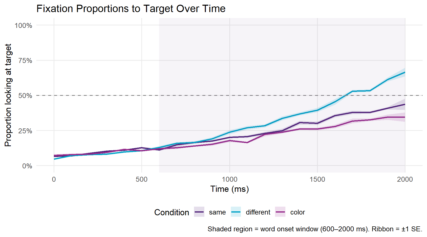
A proportion of 0.5 (the dashed line) represents chance — the participant is equally likely to be looking at the target or the competitor. Values above 0.5 indicate a target preference; values below 0.5 indicate a competitor preference.

In a typical VWP gender agreement experiment, we expect: - All conditions to start near chance (participants don’t know which image is the target yet) - The different condition to diverge earliest and most strongly above chance, because the gender mismatch on the article immediately signals which image is the target - The same condition to show a weaker or delayed target preference, because the article is compatible with both images

Participant-level spaghetti plot

A spaghetti plot shows individual participant trajectories, which helps identify outliers and assess variability.

# Aggregate by participant and time for spaghetti plot
spaghetti_dat <- response_window |>
  dplyr::group_by(participant_id, condition, Time) |>
  dplyr::summarise(mean_prop = mean(Prop, na.rm = TRUE), .groups = "drop")

ggplot(spaghetti_dat, aes(x = Time, y = mean_prop,
                           group = participant_id, colour = condition)) +
  geom_line(alpha = 0.3, linewidth = 0.4) +
  stat_summary(aes(group = condition), fun = mean,
               geom = "line", linewidth = 1.2) +
  geom_hline(yintercept = 0.5, linetype = "dashed", colour = "grey50") +
  facet_wrap(~condition) +
  scale_colour_manual(values = c("same"      = "#51247A",
                                 "different" = "#00A2C7",
                                 "color"     = "#962A8B")) +
  scale_y_continuous(limits = c(0, 1),
                     labels = scales::percent_format()) +
  labs(title   = "Individual Participant Trajectories by Condition",
       x       = "Time (ms)",
       y       = "Proportion looking at target",
       colour  = "Condition") +
  theme_minimal(base_size = 12) +
  theme(legend.position = "none",
        panel.grid.minor = element_blank())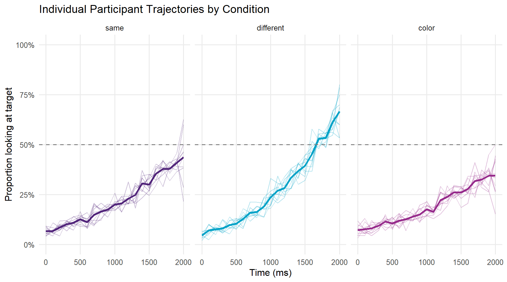

---

Statistical Analysis

Section Overview

What you will learn: How to analyse eye-tracking data using two complementary approaches — mixed-effects logistic regression on time-window aggregates, and Generalised Additive Mixed Models (GAMMs) for the full time course.

Approach 1: Mixed-Effects Logistic Regression

The most common approach to VWP analysis is to define a critical time window — typically starting at word onset and ending when the acoustic signal is complete — and aggregate fixation proportions within that window. The binary outcome (looking/not looking at target on each sample) is then modelled with logistic regression, with random effects for participants and items (Barr 2008).

This approach has both strengths and limitations. Its main strength is simplicity: a single model with interpretable coefficients answers the core question of whether conditions differ in the analysis window. Its main limitation is that the window must be chosen in advance, and different window choices can yield different conclusions. Choosing a window after inspecting the data inflates Type I error rates. The window approach also discards the time course entirely — if the different and same conditions converge at the beginning and end of the window but diverge in the middle, a window average would show no effect even though there is one. For this reason, window analysis is best used as a confirmatory test after time course visualisation has established where to look.

The critical window of 600–1800 ms used here corresponds to the period from approximate word onset to the end of the analysis epoch. This is a reasonable default for a gender agreement experiment, but the appropriate window will depend on your specific stimuli and research question.

Define the analysis window

# Define critical window (for reference — make_time_window_data aggregates
# across all time by default; filter dat_etr to the window first if needed)
window_start <- 600
window_end   <- 1800

# Filter the eyetrackingR data object to the critical window before aggregating
dat_etr_window <- dat_etr |>
  dplyr::filter(time_elapsed >= window_start, time_elapsed <= window_end)

# Now create window data from the filtered object
response_window_agg <- eyetrackingR::make_time_window_data(
  dat_etr_window,
  aois              = "AOI_target",
  predictor_columns = c("condition"),
  summarize_by      = "participant_id"
)

head(response_window_agg)

  participant_id condition SamplesInAOI SamplesTotal        AOI    Elog Weights
1            P01      same          429         1912 AOI_target -1.2395   333.1
2            P02 different          465         1533 AOI_target -0.8309   324.2
3            P03     color          383         1831 AOI_target -1.3289   303.2
4            P04      same          391         1647 AOI_target -1.1661   298.5
5            P05 different          566         1996 AOI_target -0.9263   405.8
6            P06     color          391         1885 AOI_target -1.3396   310.2
    Prop LogitAdjusted ArcSin
1 0.2244       -1.2404 0.4935
2 0.3033       -0.8315 0.5833
3 0.2092       -1.3299 0.4750
4 0.2374       -1.1670 0.5089
5 0.2836       -0.9268 0.5616
6 0.2074       -1.3405 0.4729

Fit the mixed-effects model

We model the proportion of looks to the target in the critical window as a function of condition, with random intercepts for participants and items.

# Convert proportion to counts for logistic regression
# eyetrackingR provides SamplesInAOI and SamplesTotal
response_window_agg <- response_window_agg |>
  dplyr::mutate(
    # Re-code condition with "same" as reference level
    condition = relevel(factor(condition), ref = "same")
  )

# Fit mixed-effects logistic regression
m_logistic <- lme4::glmer(
  cbind(SamplesInAOI, SamplesTotal - SamplesInAOI) ~
    condition +
    (1 | participant_id),
  data   = response_window_agg,
  family = binomial,
  control = glmerControl(optimizer = "bobyqa",
                         optCtrl   = list(maxfun = 2e5))
)

summary(m_logistic)

Generalized linear mixed model fit by maximum likelihood (Laplace
  Approximation) [glmerMod]
 Family: binomial  ( logit )
Formula: cbind(SamplesInAOI, SamplesTotal - SamplesInAOI) ~ condition +  
    (1 | participant_id)
   Data: response_window_agg
Control: glmerControl(optimizer = "bobyqa", optCtrl = list(maxfun = 200000))

     AIC      BIC   logLik deviance df.resid 
   261.8    267.4   -126.9    253.8       26 

Scaled residuals: 
   Min     1Q Median     3Q    Max 
-2.770 -0.357  0.215  0.521  2.092 

Random effects:
 Groups         Name        Variance Std.Dev.
 participant_id (Intercept) 0        0       
Number of obs: 30, groups:  participant_id, 30

Fixed effects:
                   Estimate Std. Error z value             Pr(>|z|)    
(Intercept)         -1.1800     0.0178   -66.3 < 0.0000000000000002 ***
conditiondifferent   0.2883     0.0244    11.8 < 0.0000000000000002 ***
conditioncolor      -0.1722     0.0257    -6.7       0.000000000021 ***
---
Signif. codes:  0 '***' 0.001 '**' 0.01 '*' 0.05 '.' 0.1 ' ' 1

Correlation of Fixed Effects:
            (Intr) cndtnd
cndtndffrnt -0.729       
conditinclr -0.692  0.504
optimizer (bobyqa) convergence code: 0 (OK)
boundary (singular) fit: see help('isSingular')

Visualise model estimates

sjPlot::plot_model(
  m_logistic,
  type   = "eff",
  terms  = "condition",
  title  = "Predicted Fixation Proportions by Condition",
  axis.title = c("Condition", "Proportion looking at target")
)

Interpreting the logistic model

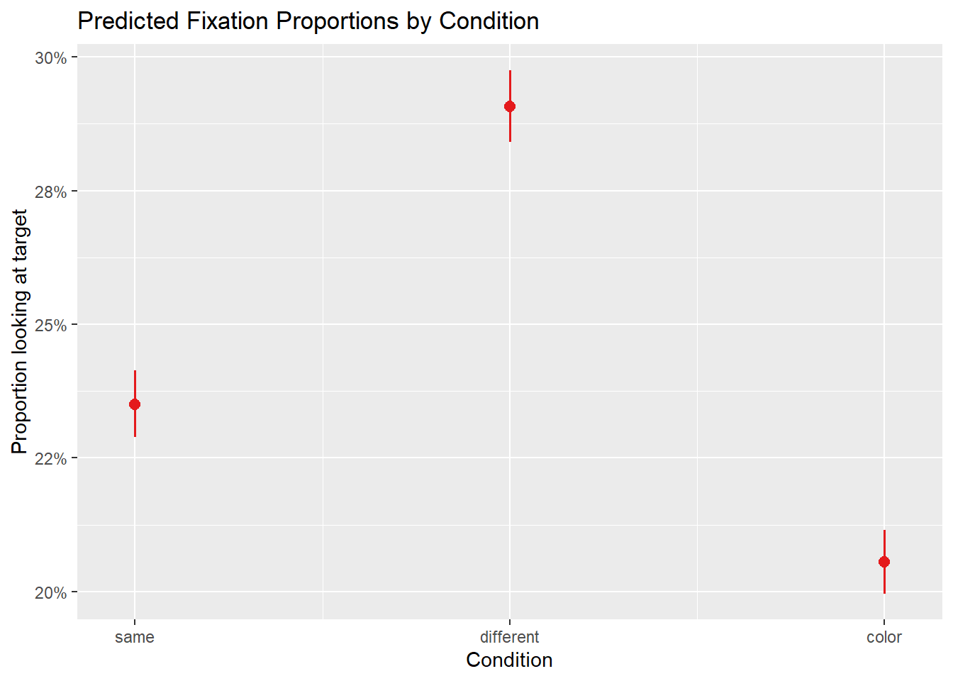
The fixed effect of condition tells us whether fixation proportions differ significantly between conditions. A positive coefficient for conditiondifferent means participants look more at the target in the different condition than in the same condition (the reference level), as we would expect if grammatical gender guides attention.

The random intercept for participant_id captures individual differences in overall target preference — some participants may be more systematic lookers than others.

Approach 2: Generalised Additive Mixed Models (GAMMs)

Mixed-effects logistic regression answers the question “do conditions differ in the analysis window?” but discards the time course entirely. Generalised Additive Mixed Models (GAMMs) offer a more powerful alternative: they model the entire trajectory of fixation proportions as a smooth function of time, allowing us to ask not just whether conditions differ, but when the difference emerges, how large it grows, and when it disappears (Wieling 2018).

GAMMs are an extension of the generalised linear model in which the relationship between a predictor and the response is represented by a smooth function (a spline) rather than a straight line. The degree of smoothness is estimated from the data rather than specified by the analyst — making GAMMs far more flexible than the polynomial terms used in growth curve analysis. This flexibility is particularly valuable for VWP data, where the time course of fixation proportions rises non-linearly from chance, plateaus, and sometimes declines again, making any fixed-order polynomial a potentially poor approximation.

Why GAMMs for eye-tracking?

The time course of fixation proportions is non-linear — it rises, plateaus, and sometimes falls back to chance — and observations at adjacent time points are highly correlated. Standard regression models assume linear effects and independent errors, both of which are violated. GAMMs handle non-linearity via smooth terms and autocorrelation via AR(1) error structures.

For a comprehensive introduction to GAMMs in linguistics, see Baayen et al. (2018) and the GAMM tutorial by Wieling (2018).

Prepare data for GAMMs

GAMMs require the data in sample-level format (not aggregated), with autocorrelation handled appropriately.

# Aggregate to participant × condition × time bin level
gamm_dat <- dat |>
  dplyr::filter(time_elapsed >= 0, time_elapsed <= 2000) |>
  dplyr::group_by(participant_id, condition, TimeBin) |>
  dplyr::summarise(
    prop_target = mean(AOI_target, na.rm = TRUE),
    n_samples   = n(),
    .groups     = "drop"
  ) |>
  dplyr::mutate(
    # Numeric participant ID for mgcv
    pid_num   = as.integer(participant_id),
    condition = relevel(factor(condition), ref = "same"),
    # Start event marker for AR1 autocorrelation
    start_event = !duplicated(paste(participant_id, condition))
  ) |>
  dplyr::arrange(participant_id, condition, TimeBin)

Fit the GAMM

# Fit GAMM with condition × time smooth interaction
# and random smooths for participants
m_gamm <- mgcv::bam(
  prop_target ~
    # Smooth of time for each condition (different smooths per condition)
    condition +
    s(TimeBin, by = condition, k = 10) +
    # Random intercept for participant
    s(participant_id, bs = "re"),
  data   = gamm_dat,
  method = "fREML",
  # AR1 autocorrelation to handle temporal dependency
  AR.start = gamm_dat$start_event,
  rho      = 0.7    # autocorrelation parameter (estimate from data in practice)
)

summary(m_gamm)

Family: gaussian 
Link function: identity 

Formula:
prop_target ~ condition + s(TimeBin, by = condition, k = 10) + 
    s(participant_id, bs = "re")

Parametric coefficients:
                   Estimate Std. Error t value             Pr(>|t|)    
(Intercept)         0.22052    0.00978   22.56 < 0.0000000000000002 ***
conditiondifferent  0.05656    0.01386    4.08             0.000051 ***
conditioncolor     -0.02832    0.01379   -2.05                 0.04 *  
---
Signif. codes:  0 '***' 0.001 '**' 0.01 '*' 0.05 '.' 0.1 ' ' 1

Approximate significance of smooth terms:
                                    edf Ref.df     F             p-value    
s(TimeBin):conditionsame      2.4508669   3.17  67.6 <0.0000000000000002 ***
s(TimeBin):conditiondifferent 3.8024045   4.92 120.1 <0.0000000000000002 ***
s(TimeBin):conditioncolor     1.9365145   2.49  50.0 <0.0000000000000002 ***
s(participant_id)             0.0000182  27.00   0.0                   1    
---
Signif. codes:  0 '***' 0.001 '**' 0.01 '*' 0.05 '.' 0.1 ' ' 1

R-sq.(adj) =  0.928   Deviance explained = 92.9%
fREML = -1011.3  Scale est. = 0.0041507  n = 630

Setting the autocorrelation parameter

The rho parameter above is set to 0.7 for illustration. In practice, you should estimate it from the data using itsadug::start_value_rho() on a model fitted without AR1 correction first:

# Step 1: fit without AR1
m_gamm_noar <- mgcv::bam(prop_target ~ condition + s(TimeBin, by = condition, k = 10) +
                           s(participant_id, bs = "re"), data = gamm_dat, method = "fREML")
# Step 2: estimate rho
rho_estimate <- itsadug::start_value_rho(m_gamm_noar)
# Step 3: refit with AR1
m_gamm <- mgcv::bam(..., rho = rho_estimate, AR.start = gamm_dat$start_event)

Visualise GAMM smooth terms

# Create prediction grid
pred_grid <- expand.grid(
  TimeBin        = seq(0, 2000, by = 50),
  condition      = levels(gamm_dat$condition),
  participant_id = levels(gamm_dat$participant_id)[1]  # reference participant
)

pred_grid$fit <- predict(m_gamm, newdata = pred_grid,
                         exclude = "s(participant_id)", se.fit = FALSE)

ggplot(pred_grid, aes(x = TimeBin, y = fit,
                      colour = condition, fill = condition)) +
  geom_line(linewidth = 1) +
  geom_hline(yintercept = 0.5, linetype = "dashed", colour = "grey50") +
  annotate("rect", xmin = 600, xmax = 2000,
           ymin = -Inf, ymax = Inf, alpha = 0.05, fill = "#51247A") +
  scale_colour_manual(values = c("same"      = "#51247A",
                                 "different" = "#00A2C7",
                                 "color"     = "#962A8B")) +
  scale_fill_manual(values   = c("same"      = "#51247A",
                                 "different" = "#00A2C7",
                                 "color"     = "#962A8B")) +
  scale_y_continuous(limits = c(0, 1),
                     labels = scales::percent_format()) +
  labs(title   = "GAMM-Predicted Fixation Proportions Over Time",
       x       = "Time (ms)",
       y       = "Predicted proportion looking at target",
       colour  = "Condition",
       fill    = "Condition",
       caption = "Shaded region = word onset window. Predictions exclude random effects.") +
  theme_minimal(base_size = 13) +
  theme(legend.position = "bottom",
        panel.grid.minor = element_blank())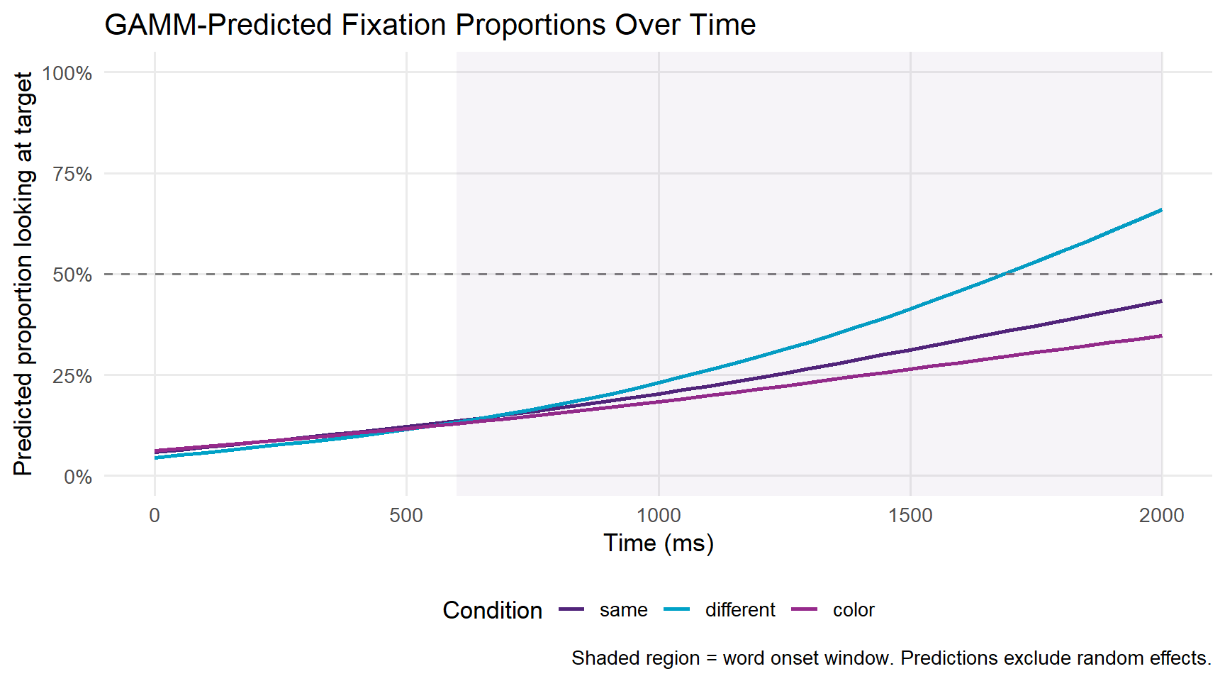

Test for significant differences between conditions

A key advantage of GAMMs is that we can test whether the smooth for one condition differs significantly from another using difference smooths.

# Use itsadug to plot the difference smooth between conditions
# This shows WHERE in time the conditions are significantly different
itsadug::plot_diff(
  m_gamm,
  view    = "TimeBin",
  comp    = list(condition = c("different", "same")),
  main    = "Difference: different vs. same condition",
  ylab    = "Difference in fixation proportion",
  xlab    = "Time (ms)",
  col     = "#00A2C7",
  shade   = TRUE
)

Summary:
    * TimeBin : numeric predictor; with 100 values ranging from 0.000000 to 2000.000000. 
    * participant_id : factor; set to the value(s): P01. (Might be canceled as random effect, check below.) 
    * NOTE : The following random effects columns are canceled: s(participant_id)
 

TimeBin window(s) of significant difference(s):
    1111.111111 - 2000.000000

abline(h = 0, lty = 2, col = "grey50")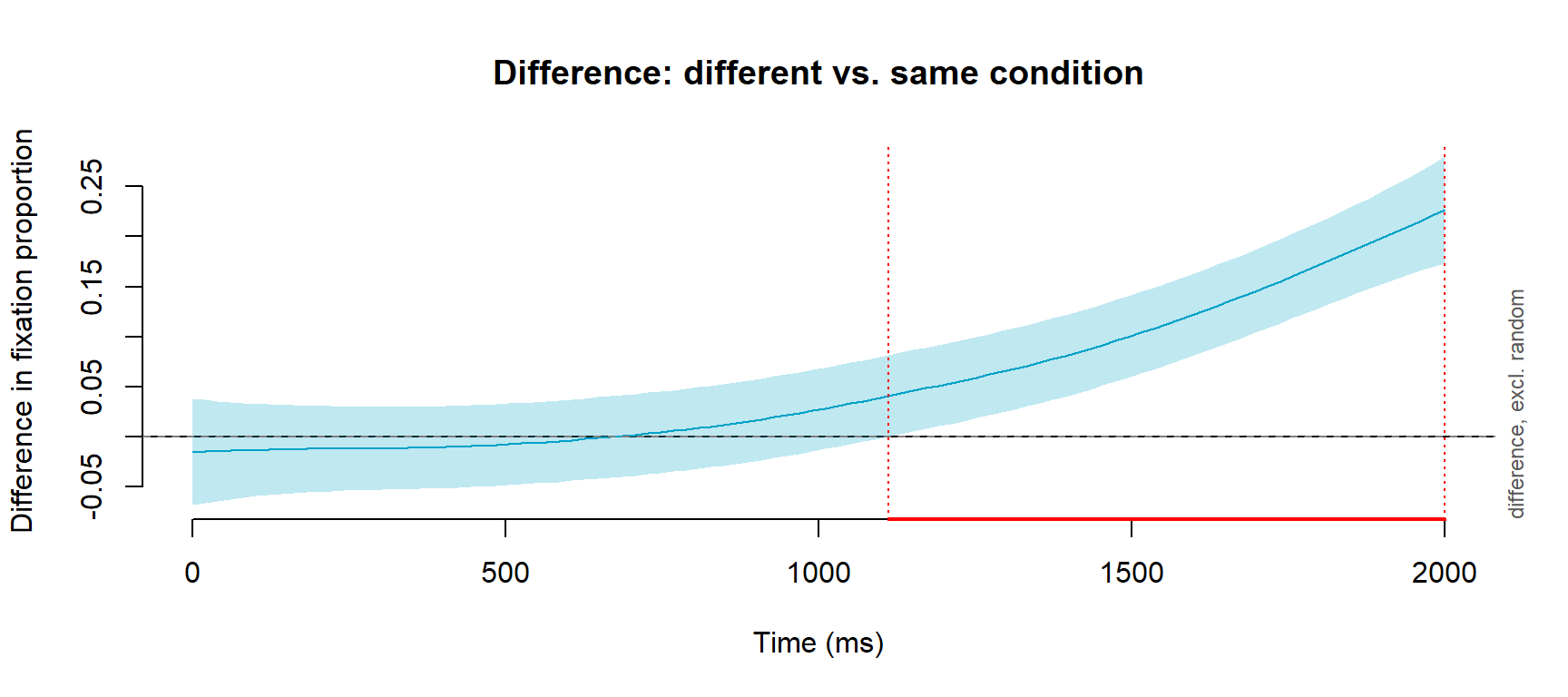

Interpreting the difference smooth

The difference smooth shows the estimated difference between the different and same conditions at each time point. When the shaded confidence interval does not include zero, the conditions are significantly different at that point in time. This allows you to make precise, data-driven statements about when a condition effect emerges — for example “conditions diverged significantly from 750 ms onwards.”

---

Growth Curve Analysis

Section Overview

What you will learn: How to perform Growth Curve Analysis (GCA), a mixed-effects polynomial regression approach to VWP time course data that is widely used in the psycholinguistics literature.

Growth Curve Analysis (GCA) (Mirman 2014) was developed specifically for the analysis of VWP time course data. The approach uses orthogonal polynomial time terms — a linear term capturing the overall rise in target fixations, a quadratic term capturing the curvature of that rise, and sometimes higher-order terms — within a standard mixed-effects regression framework (Mirman, Dixon, and Magnuson 2008). The key advantage of GCA over time-window analysis is that it retains and models the time course rather than collapsing it, while remaining within the familiar mixed-effects regression framework that most psycholinguists already know.

GCA is particularly well suited to capturing the characteristic S-shaped trajectory of VWP data: fixation proportions start near chance, rise steeply as the acoustic signal disambiguates, and then plateau at a high level. The linear term captures the overall direction of change, and the quadratic term captures whether the rise is accelerating (convex) or decelerating (concave). Experimental effects are reflected in interactions between these polynomial time terms and the condition predictor — for example, a significant ot1:condition interaction indicates that one condition shows a steeper overall rise than another, while a significant ot2:condition interaction indicates that the shape of the rise differs between conditions.

GCA is a useful complement to GAMMs when you want interpretable, directly comparable coefficients (for reporting in tables or comparing across studies) rather than flexible smooths.

# Create orthogonal polynomial time terms
# Using the analysis window 600–1800 ms
gca_dat <- dat |>
  dplyr::filter(time_elapsed >= 600, time_elapsed <= 1800) |>
  dplyr::group_by(participant_id, condition, TimeBin) |>
  dplyr::summarise(
    prop_target = mean(AOI_target, na.rm = TRUE),
    .groups     = "drop"
  ) |>
  dplyr::mutate(
    condition = relevel(factor(condition), ref = "same")
  )

# Create orthogonal polynomial time terms (linear + quadratic)
t <- poly(unique(gca_dat$TimeBin), 2)
gca_dat[, c("ot1", "ot2")] <- t[match(gca_dat$TimeBin,
                                        unique(gca_dat$TimeBin)), 1:2]

# Fit growth curve model
m_gca <- lme4::lmer(
  prop_target ~
    # Fixed effects: condition × time interactions
    (ot1 + ot2) * condition +
    # Random effects: participant-level time course variation
    (ot1 + ot2 | participant_id),
  data    = gca_dat,
  REML    = FALSE,
  control = lmerControl(optimizer = "bobyqa")
)

summary(m_gca)

Linear mixed model fit by maximum likelihood  ['lmerMod']
Formula: prop_target ~ (ot1 + ot2) * condition + (ot1 + ot2 | participant_id)
   Data: gca_dat
Control: lmerControl(optimizer = "bobyqa")

     AIC      BIC   logLik deviance df.resid 
 -1348.5  -1286.3    690.2  -1380.5      344 

Scaled residuals: 
   Min     1Q Median     3Q    Max 
-2.686 -0.716 -0.019  0.666  3.277 

Random effects:
 Groups         Name        Variance   Std.Dev. Corr       
 participant_id (Intercept) 0.00000886 0.00298             
                ot1         0.00002182 0.00467   0.49      
                ot2         0.00010590 0.01029  -0.81  0.12
 Residual                   0.00124676 0.03531             
Number of obs: 360, groups:  participant_id, 30

Fixed effects:
                       Estimate Std. Error t value
(Intercept)             0.23523    0.00336   70.05
ot1                     0.27452    0.01126   24.37
ot2                     0.03239    0.01163    2.79
conditiondifferent      0.05732    0.00475   12.07
conditioncolor         -0.03057    0.00475   -6.44
ot1:conditiondifferent  0.13810    0.01593    8.67
ot1:conditioncolor     -0.05828    0.01593   -3.66
ot2:conditiondifferent  0.02817    0.01645    1.71
ot2:conditioncolor     -0.01418    0.01645   -0.86

Correlation of Fixed Effects:
            (Intr) ot1    ot2    cndtnd cndtnc ot1:cndtnd ot1:cndtnc ot2:cndtnd
ot1          0.018                                                             
ot2         -0.064  0.004                                                      
cndtndffrnt -0.707 -0.013  0.045                                               
conditinclr -0.707 -0.013  0.045  0.500                                        
ot1:cndtndf -0.013 -0.707 -0.003  0.018  0.009                                 
ot1:cndtncl -0.013 -0.707 -0.003  0.009  0.018  0.500                          
ot2:cndtndf  0.045 -0.003 -0.707 -0.064 -0.032  0.004      0.002               
ot2:cndtncl  0.045 -0.003 -0.707 -0.032 -0.064  0.002      0.004      0.500    
optimizer (bobyqa) convergence code: 0 (OK)
boundary (singular) fit: see help('isSingular')

# Plot observed vs. model-predicted trajectories
# Join fitted values onto gca_dat, then summarise by condition and time bin
gca_plot_dat <- gca_dat |>
  dplyr::mutate(fitted = fitted(m_gca)) |>
  dplyr::group_by(condition, TimeBin) |>
  dplyr::summarise(
    mean_obs  = mean(prop_target, na.rm = TRUE),
    mean_pred = mean(fitted,      na.rm = TRUE),
    .groups   = "drop"
  )

gca_plot_dat |>
  ggplot(aes(x = TimeBin, colour = condition)) +
  geom_point(aes(y = mean_obs), alpha = 0.5, size = 1.5) +
  geom_line(aes(y = mean_pred), linewidth = 1) +
  geom_hline(yintercept = 0.5, linetype = "dashed", colour = "grey50") +
  scale_colour_manual(values = c("same"      = "#51247A",
                                 "different" = "#00A2C7",
                                 "color"     = "#962A8B")) +
  scale_y_continuous(limits = c(0, 1),
                     labels = scales::percent_format()) +
  labs(title   = "Growth Curve Analysis: Observed vs. Predicted",
       x       = "Time (ms)",
       y       = "Proportion looking at target",
       colour  = "Condition",
       caption = "Points = observed means; lines = GCA model predictions.") +
  theme_minimal(base_size = 13) +
  theme(legend.position = "bottom",
        panel.grid.minor = element_blank())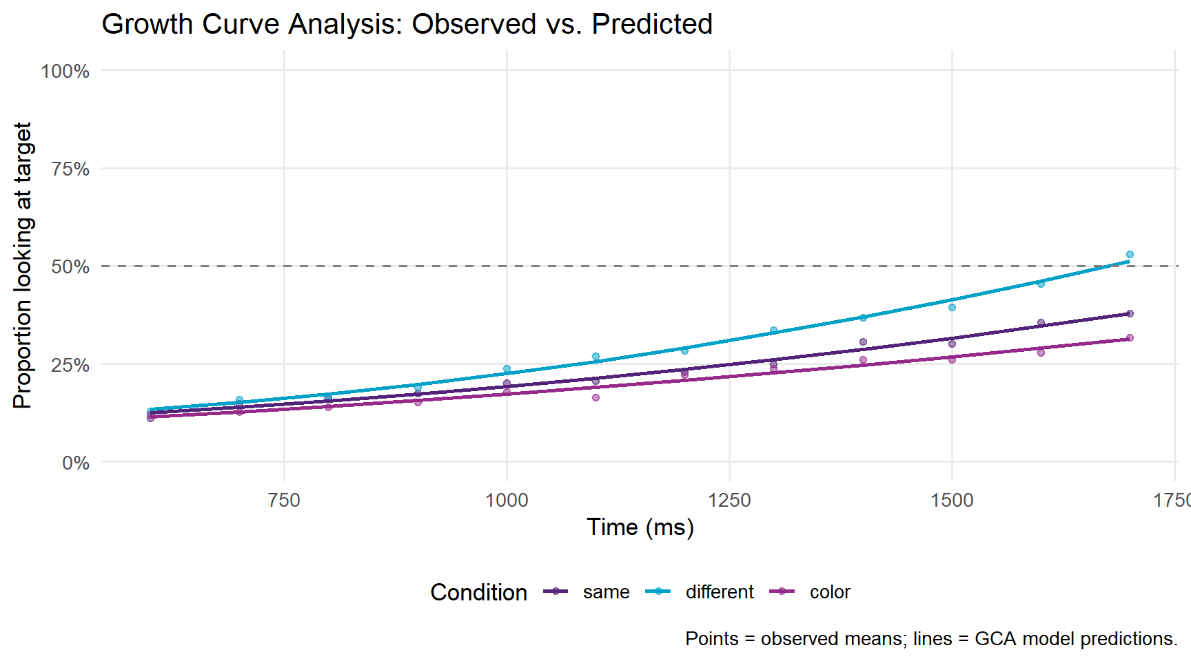

---

Summary and Recommendations

This tutorial has walked through the complete workflow for processing and analysing Visual World Paradigm eye-tracking data in R:

Processing:

1. Load and combine participant data files and trial metadata
2. Apply confidence thresholds to exclude low-quality gaze samples
3. Code Areas of Interest (AOIs) from coordinate data
4. Bin continuous gaze data into 100 ms time windows
5. Clean data by fixing labelling errors and removing incorrect trials

Analysis:

6. Create an eyetrackingR data object for validated processing
7. Visualise fixation proportion time courses by condition
8. Fit mixed-effects logistic regression on critical time window aggregates
9. Fit GAMMs to model the full time course with non-linear smooths
10. Use Growth Curve Analysis for interpretable polynomial time effects

Choosing between analytical approaches:

Method	Best for	Limitation
Mixed-effects logistic regression	Testing condition effects in a pre-defined window	Discards time course; window choice is arbitrary
GAMMs	Modelling full time course; identifying when effects emerge	More complex to fit and interpret
Growth Curve Analysis	Interpretable time course effects; comparison with published GCA literature	Assumes polynomial shape; less flexible than GAMMs

In practice, many researchers use all three — logistic regression for a simple confirmatory test, GAMMs for exploratory time course analysis, and GCA for compatibility with the broader literature.

Citation & Session Info

Citation

Martin Schweinberger. 2026. Processing and Analysing Eye-Tracking Data in R. The Language Technology and Data Analysis Laboratory (LADAL), The University of Queensland, Australia. url: https://ladal.edu.au/tutorials/eyetracking/eyetracking.html (Version 2026.03.31), doi: .

@manual{martinschweinberger2026processing,
  author       = {Martin Schweinberger},
  title        = {Processing and Analysing Eye-Tracking Data in R},
  year         = {2026},
  note         = {https://ladal.edu.au/tutorials/eyetracking/eyetracking.html},
  organization = {The Language Technology and Data Analysis Laboratory (LADAL), The University of Queensland, Australia},
  edition      = {2026.03.31},
  doi          = {}
}

sessionInfo()

R version 4.4.2 (2024-10-31 ucrt)
Platform: x86_64-w64-mingw32/x64
Running under: Windows 11 x64 (build 26200)

Matrix products: default


locale:
[1] LC_COLLATE=English_United States.utf8 
[2] LC_CTYPE=English_United States.utf8   
[3] LC_MONETARY=English_United States.utf8
[4] LC_NUMERIC=C                          
[5] LC_TIME=English_United States.utf8    

time zone: Australia/Brisbane
tzcode source: internal

attached base packages:
[1] stats     graphics  grDevices datasets  utils     methods   base     

other attached packages:
 [1] here_1.0.2         sjPlot_2.8.17      lme4_1.1-36        Matrix_1.7-2      
 [5] itsadug_2.5        plotfunctions_1.5  mgcv_1.9-1         nlme_3.1-166      
 [9] data.table_1.17.0  eyetrackingR_0.2.2 lubridate_1.9.4    forcats_1.0.0     
[13] stringr_1.6.0      dplyr_1.2.0        purrr_1.2.1        readr_2.1.5       
[17] tidyr_1.3.2        tibble_3.3.1       ggplot2_4.0.2      tidyverse_2.0.0   
[21] checkdown_0.0.13  

loaded via a namespace (and not attached):
 [1] tidyselect_1.2.1    sjlabelled_1.2.0    farver_2.1.2       
 [4] S7_0.2.1            fastmap_1.2.0       lazyeval_0.2.2     
 [7] sjstats_0.19.0      digest_0.6.39       estimability_1.5.1 
[10] timechange_0.3.0    lifecycle_1.0.5     survival_3.7-0     
[13] magrittr_2.0.4      compiler_4.4.2      rlang_1.1.7        
[16] tools_4.4.2         yaml_2.3.10         knitr_1.51         
[19] labeling_0.4.3      htmlwidgets_1.6.4   RColorBrewer_1.1-3 
[22] withr_3.0.2         effects_4.2-2       nnet_7.3-19        
[25] grid_4.4.2          datawizard_1.3.0    colorspace_2.1-1   
[28] scales_1.4.0        MASS_7.3-61         insight_1.4.6      
[31] cli_3.6.5           survey_4.4-2        rmarkdown_2.30     
[34] reformulas_0.4.0    generics_0.1.4      rstudioapi_0.17.1  
[37] performance_0.16.0  tzdb_0.5.0          minqa_1.2.8        
[40] DBI_1.2.3           splines_4.4.2       BiocManager_1.30.27
[43] mitools_2.4         vctrs_0.7.2         boot_1.3-31        
[46] jsonlite_2.0.0      carData_3.0-5       hms_1.1.4          
[49] glue_1.8.0          nloptr_2.1.1        codetools_0.2-20   
[52] stringi_1.8.7       gtable_0.3.6        ggeffects_2.2.0    
[55] pillar_1.11.1       htmltools_0.5.9     R6_2.6.1           
[58] Rdpack_2.6.2        rprojroot_2.1.1     evaluate_1.0.5     
[61] lattice_0.22-6      markdown_2.0        rbibutils_2.3      
[64] snakecase_0.11.1    renv_1.1.7          Rcpp_1.1.1         
[67] xfun_0.56           sjmisc_2.8.10       pkgconfig_2.0.3    

AI Transparency Statement

This tutorial was re-developed with the assistance of Claude (claude.ai), a large language model created by Anthropic. Claude was used to help revise the tutorial text, structure the instructional content, generate the R code examples, and write the checkdown quiz questions and feedback strings. All content was reviewed, edited, and approved by the author (Martin Schweinberger), who takes full responsibility for the accuracy and pedagogical appropriateness of the material. The use of AI assistance is disclosed here in the interest of transparency and in accordance with emerging best practices for AI-assisted academic content creation.

Back to top Back to HOME

References

Allopenna, Paul D., James S. Magnuson, and Michael K. Tanenhaus. 1998. “Tracking the Time Course of Spoken Word Recognition Using Eye Movements: Evidence for Continuous Mapping Models.” Journal of Memory and Language 38 (4): 419–39. https://doi.org/10.1006/jmla.1997.2558.

Barr, Dale J. 2008. “Analyzing ‘Visual World’ Eyetracking Data Using Multilevel Logistic Regression.” Journal of Memory and Language 59 (4): 457–74. https://doi.org/10.1016/j.jml.2007.09.002.

Dahan, Delphine, Daniel Swingley, Michael K. Tanenhaus, and James S. Magnuson. 2000. “Linguistic Gender and Spoken-Word Recognition in French.” Journal of Memory and Language 42 (4): 465–80. https://doi.org/10.1006/jmla.1999.2688.

Mirman, Daniel. 2014. Growth Curve Analysis and Visualization Using R. Boca Raton, FL: Chapman; Hall/CRC.

Mirman, Daniel, James A. Dixon, and James S. Magnuson. 2008. “Statistical and Computational Models of the Visual World Paradigm: Growth Curves and Individual Differences.” Journal of Memory and Language 59 (4): 475–94. https://doi.org/10.1016/j.jml.2007.11.006.

Tanenhaus, Michael K., Michael J. Spivey-Knowlton, Kathleen M. Eberhard, and Julie C. Sedivy. 1995. “Integration of Visual and Linguistic Information in Spoken Language Comprehension.” Science 268 (5217): 1632–34. https://doi.org/10.1126/science.7777863.

Wieling, Martijn. 2018. “Analyzing Dynamic Phonetic Data Using Generalized Additive Mixed Modeling: A Tutorial Focusing on Articulatory Differences Between L1 and L2 Speakers of English.” Journal of Phonetics 70: 86–116. https://doi.org/10.1016/j.wocn.2018.03.002.