Basic Inferential Statistics using R

Great Court, The University of Queensland

Introduction

This tutorial introduces basic inferential statistics — the methods we use to draw conclusions about populations based on samples, test hypotheses, and quantify the strength and significance of relationships in data. Where descriptive statistics summarise what we observe, inferential statistics allow us to reason about what we cannot directly observe: the patterns and relationships that exist in the broader population our data represent.

Inferential statistics provide an indispensable framework for empirical research in linguistics and the humanities. They help us determine whether an observed difference between groups (e.g., native speakers vs. learners) is likely to reflect a genuine population-level difference or whether it could plausibly have arisen by chance. They also help us quantify the strength of associations, assess the reliability of our estimates, and communicate uncertainty honestly.

This tutorial is aimed at beginners and intermediate R users. The goal is not to provide a fully comprehensive treatment of statistics but to introduce and exemplify the most commonly used inferential tests in linguistics research, covering both their conceptual foundations and their implementation in R.

Learning Objectives

By the end of this tutorial you will be able to:

1. Explain the logic of null hypothesis significance testing (NHST) and correctly interpret p-values and effect sizes
2. Check parametric assumptions visually (histograms, Q-Q plots) and formally (Shapiro-Wilk, Levene’s test)
3. Compute and interpret skewness and kurtosis
4. Decide between parametric and non-parametric tests based on data characteristics
5. Apply paired and independent t-tests in R and extract Cohen’s d as an effect size
6. Apply Fisher’s Exact Test, Mann-Whitney U, Wilcoxon signed rank, Kruskal-Wallis, and Friedman tests
7. Perform Pearson’s χ² test and compute phi or Cramér’s V as effect sizes
8. Apply chi-square extensions for 2×k and z×k sub-tables
9. Conduct Configural Frequency Analysis (CFA) and Hierarchical CFA (HCFA)
10. Report inferential statistics in APA style with test statistics, degrees of freedom, p-values, and effect sizes

Prerequisite Tutorials

Before working through this tutorial, we recommend familiarity with the following:

• Introduction to Quantitative Reasoning
• Basic Concepts in Quantitative Research
• Descriptive Statistics
• Introduction to Data Visualization
• Data Visualization with R
• Getting started with R
• Loading, saving, and generating data in R
• Handling Tables in R

Citation

Martin Schweinberger. 2026. Basic Inferential Statistics using R. The Language Technology and Data Analysis Laboratory (LADAL), The University of Queensland, Australia. url: https://ladal.edu.au/tutorials/inferential_stats/inferential_stats.html (Version 3.1.1).

Preparation and Session Set-up

Install required packages once:

install.packages("dplyr")
install.packages("ggplot2")
install.packages("tidyr")
install.packages("flextable")
install.packages("e1071")
install.packages("lawstat")
install.packages("fGarch")
install.packages("gridExtra")
install.packages("cfa")
install.packages("effectsize")
install.packages("report")
install.packages("checkdown")

Load packages for this session:

library(dplyr)       # data processing
library(ggplot2)     # data visualisation
library(tidyr)       # data transformation
library(flextable)   # formatted tables
library(e1071)       # skewness and kurtosis
library(lawstat)     # Levene's test
library(fGarch)      # skewed distributions
library(gridExtra)   # multi-panel plots
library(cfa)         # configural frequency analysis
library(effectsize)  # effect size measures
library(report)      # automated result summaries
library(checkdown)   # interactive exercises

Load the sample datasets used throughout this tutorial:

itdata  <- base::readRDS("tutorials/inferential_stats/data/itdata.rda", "rb")
ptdata  <- base::readRDS("tutorials/inferential_stats/data/ptdata.rda", "rb")
fedata  <- base::readRDS("tutorials/inferential_stats/data/fedata.rda", "rb")
mwudata <- base::readRDS("tutorials/inferential_stats/data/mwudata.rda", "rb")
uhmdata <- base::readRDS("tutorials/inferential_stats/data/uhmdata.rda", "rb")
frdata  <- base::readRDS("tutorials/inferential_stats/data/frdata.rda", "rb")
x2data  <- base::readRDS("tutorials/inferential_stats/data/x2data.rda", "rb")
x2edata <- base::readRDS("tutorials/inferential_stats/data/x2edata.rda", "rb")
mdata   <- base::readRDS("tutorials/inferential_stats/data/mdata.rda", "rb")

---

Inferential Logic: From Sample to Population

Section Overview

What you will learn: The conceptual foundation of inferential statistics — what a p-value actually means, how NHST works, and why effect sizes are essential alongside significance tests.

When we collect data in linguistics — a corpus, an experiment, a survey — we almost never observe the entire population of interest. Instead, we work with a sample: a subset of the population we hope is representative. Inferential statistics provide the tools to reason from the sample to the population under conditions of uncertainty.

The dominant framework for this reasoning is null hypothesis significance testing (NHST):

1. We formulate a null hypothesis (H₀) — typically that there is no effect, no difference, or no association in the population.
2. We formulate an alternative hypothesis (H₁) — the substantive claim we want to test.
3. We calculate a test statistic that summarises how far our data deviate from what H₀ would predict.
4. We compute a p-value: the probability of observing a test statistic as extreme as ours (or more extreme) if H₀ were true.
5. If p falls below a pre-specified significance threshold (typically α = .05), we reject H₀ in favour of H₁.

Common misconceptions about p-values

The p-value is one of the most frequently misinterpreted statistics in all of science. It is not:

• The probability that H₀ is true
• The probability that the result is due to chance
• A measure of the size or importance of an effect
• A guarantee of reproducibility

A p-value below .05 tells us only that our data are unlikely under H₀. It says nothing about the magnitude of the effect (which requires an effect size) or whether the result will replicate (which requires power and replication).

Always report effect sizes alongside p-values.

Parametric vs. non-parametric tests

Tests can be broadly divided into two families:

Type	When to use	Examples
Parametric	Data (or residuals) are approximately normally distributed; numeric dependent variable	t-test, ANOVA, linear regression
Non-parametric	Data are ordinal, or residuals are non-normal; robust to assumption violations	Mann-Whitney U, Wilcoxon, Kruskal-Wallis, χ²

The choice between parametric and non-parametric tests depends on whether parametric assumptions are met — which is what we turn to next.

---

Checking Assumptions

Section Overview

What you will learn: How to assess whether your data meet the assumptions required for parametric tests.

Key methods: Visual inspection (histograms, Q-Q plots), skewness, kurtosis, Shapiro-Wilk test, Levene’s test

Why it matters: Using a parametric test on data that violate its assumptions can produce misleading results.

The most important assumptions for parametric tests are:

1. Normality: The errors (residuals) within each group are approximately normally distributed
2. Homogeneity of variances (homoskedasticity): The variances of the groups are approximately equal

We illustrate assumption checking with word count data from a sample corpus, extracting 100 utterances from men and 100 from women.

ndata <- mdata |>
  dplyr::rename(Gender = sex, Words = word.count) |>
  dplyr::select(Gender, Words) |>
  dplyr::filter(!is.na(Words), !is.na(Gender)) |>
  dplyr::group_by(Gender) |>
  dplyr::sample_n(100)

Gender	Words
female	410
female	242
female	1,310
female	814
female	443
female	769
female	638
female	43
female	445
female	4

---

Visual inspection

Histograms

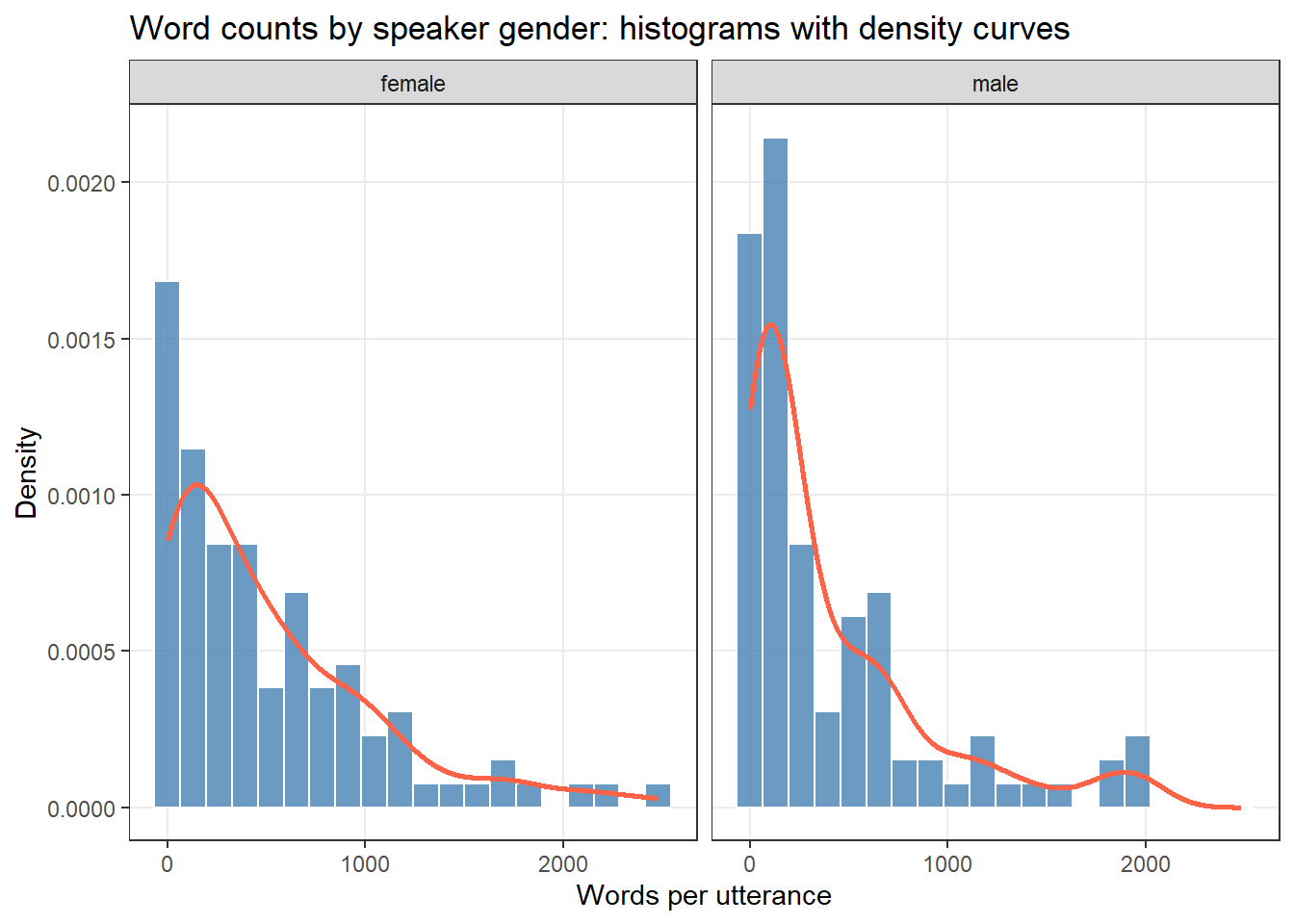
Histograms with density curves give an immediate impression of the distribution shape. A normally distributed variable should produce a symmetric, bell-shaped histogram.

ggplot(ndata, aes(x = Words)) +
  facet_grid(~Gender) +
  geom_histogram(aes(y = after_stat(density)), bins = 20,
                 fill = "steelblue", color = "white", alpha = 0.8) +
  geom_density(color = "tomato", linewidth = 1) +
  theme_bw() +
  labs(title = "Word counts by speaker gender: histograms with density curves",
       x = "Words per utterance", y = "Density") +
  theme(panel.grid.minor = element_blank())

The strong right skew in both groups suggests non-normality — a very common pattern in linguistic data, where a few very long utterances dominate the upper tail.

Quantile-quantile plots

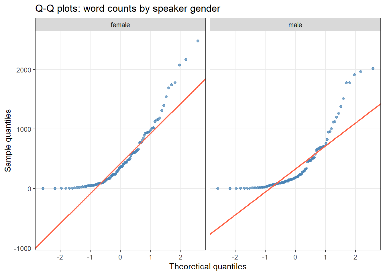
A Q-Q plot compares the quantiles of the observed data against quantiles expected from a normal distribution. If the data are normal, points fall along the diagonal reference line. Departures from the line — especially systematic curves — indicate non-normality.

ggplot(ndata, aes(sample = Words)) +
  facet_grid(~Gender) +
  geom_qq(color = "steelblue", alpha = 0.7) +
  geom_qq_line(color = "tomato", linewidth = 0.8) +
  theme_bw() +
  labs(title = "Q-Q plots: word counts by speaker gender",
       x = "Theoretical quantiles", y = "Sample quantiles") +
  theme(panel.grid.minor = element_blank())

The upward curve at the right tail confirms positive skew (a longer-than-normal upper tail) in both groups.

---

Statistical measures: skewness and kurtosis

Skewness

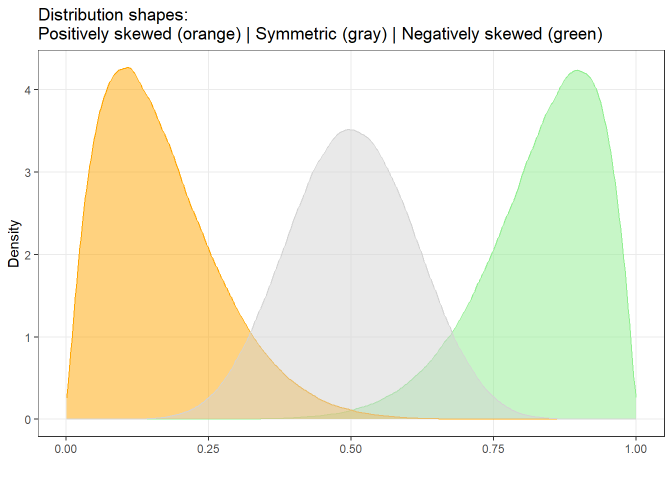
Skewness measures the asymmetry of a distribution. In a perfectly symmetric distribution, skewness = 0. When the tail extends to the right, we have positive (right) skew; when it extends to the left, we have negative (left) skew.

As a rule of thumb, skewness values outside the range [−1, +1] indicate substantial skew that may violate parametric assumptions.

words_women <- ndata |>
  dplyr::filter(Gender == "female") |>
  dplyr::pull(Words)

summary(words_women)

   Min. 1st Qu.  Median    Mean 3rd Qu.    Max. 
   0.00   89.75  359.00  510.98  771.00 2482.00 

The mean is considerably larger than the median, confirming positive skew. We quantify it using the skewness() function from the e1071 package:

e1071::skewness(words_women, type = 2)

[1] 1.49985700164

Interpreting skewness values

Skewness	Interpretation
−0.5 to +0.5	Approximately symmetric
−1 to −0.5 or +0.5 to +1	Moderate skew
< −1 or > +1	Substantial skew — parametric assumptions likely violated

Positive skewness means the distribution leans left (the tail points right). Negative skewness means the distribution leans right (the tail points left).

Kurtosis

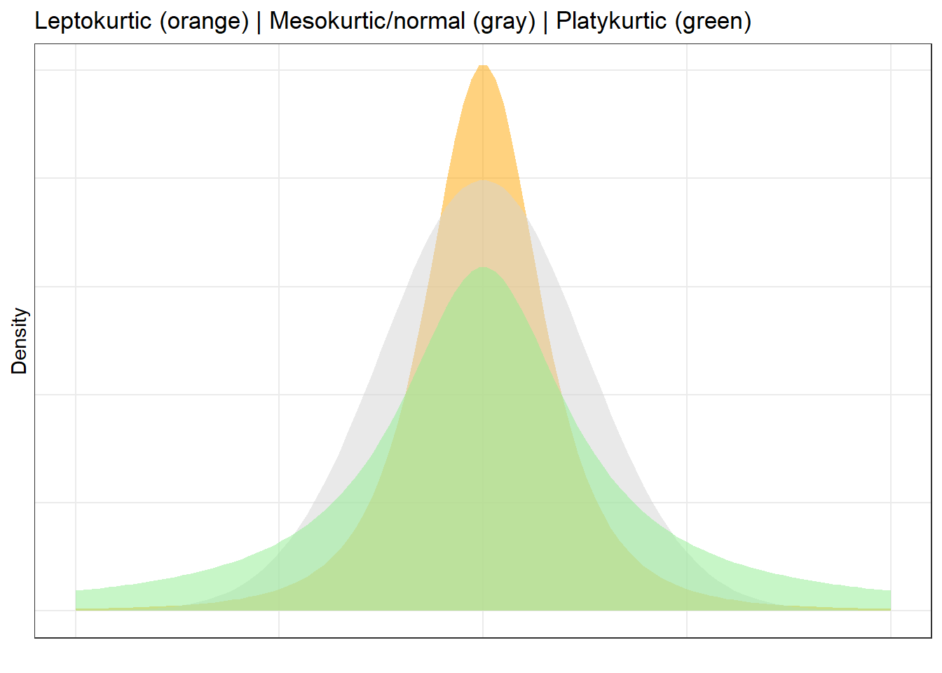
Kurtosis measures the peakedness and tail weight of a distribution relative to the normal distribution. Three types are commonly distinguished:

• Mesokurtic: Normal-like (excess kurtosis ≈ 0)
• Leptokurtic: Taller peak and heavier tails than normal (excess kurtosis > 0)
• Platykurtic: Flatter peak and thinner tails than normal (excess kurtosis < 0)

e1071::kurtosis(words_women)

[1] 1.90608160299

A kurtosis value above 1 indicates leptokurtosis (too peaked); below −1 indicates platykurtosis (too flat).

---

Formal tests of assumptions

Shapiro-Wilk test

The Shapiro-Wilk test formally tests H₀: “the data are normally distributed.” A p-value greater than .05 means we cannot reject normality; a p-value below .05 indicates significant departure from normality.

Shapiro-Wilk: limitations

The Shapiro-Wilk test is sensitive to sample size:

• Small samples (n < 50): Low power — may fail to detect genuine non-normality
• Large samples (n > 200): Overly strict — flags trivially small deviations as significant

Always use the Shapiro-Wilk test alongside visual inspection, not as the sole criterion.

shapiro.test(words_women)

    Shapiro-Wilk normality test

data:  words_women
W = 0.8388897344, p-value = 0.00000000470750796

The test confirms significant departure from normality (W = 0.79, p < .001), suggesting a non-parametric test may be more appropriate.

Levene’s test

The Levene’s test tests H₀: “the variances of the groups are equal” (homoskedasticity). Unequal variances can undermine the reliability of parametric tests that assume equal group variances.

lawstat::levene.test(mdata$word.count, mdata$sex)

    Modified robust Brown-Forsythe Levene-type test based on the absolute
    deviations from the median

data:  mdata$word.count
Test Statistic = 0.005008415511, p-value = 0.943592186

Here (W ≈ 0.005, p = .944), the variances of men and women are approximately equal — we cannot reject homoskedasticity.

Deciding between parametric and non-parametric tests

Use this decision tree:

1. Is the dependent variable numeric (interval or ratio scale)? No → non-parametric
2. Are the residuals within each group approximately normal? No → consider non-parametric
3. Are the variances approximately equal? No → consider Welch’s t-test or non-parametric

When in doubt, run both and compare conclusions. If they agree, the violation may not be consequential. If they disagree, prefer the non-parametric result.

---

Exercises: Checking Assumptions

Q1. A Q-Q plot shows data points falling closely along the diagonal line in the centre, but curving sharply upward at the right end. What does this indicate?

Right skew — the upper tail is longer than a normal distribution would predict
Left skew — the lower tail is longer than normal
The data are approximately normally distributed
Leptokurtosis — the distribution is too peaked

Q2. A Shapiro-Wilk test returns W = 0.99, p = .62 for a sample of n = 500. Can you safely conclude that the data are normally distributed?

The test is invalid for samples larger than n = 100
Not definitively — with large samples the Shapiro-Wilk test is underpowered to detect small, practically inconsequential deviations, so visual inspection is still needed
Yes — p > .05 confirms normality beyond doubt
No — p > .05 means we must reject the normality assumption

Q3. A Levene’s test returns p = .018. What should you do next?

Remove the group with higher variance from the analysis
Increase the sample size until Levene's test is non-significant
Proceed with Student's t-test as usual — Levene's test is just advisory
Consider using Welch's t-test (which does not assume equal variances) rather than Student's t-test, or switch to a non-parametric alternative

---

Parametric Tests

Section Overview

What you will learn: When and how to apply t-tests and extract effect sizes in R.

Prerequisites: Normally distributed residuals within each group; numeric dependent variable

Key tests: Paired t-test, independent t-test (Student’s and Welch’s)

Parametric tests assume that the residuals (errors) within each group are approximately normally distributed. They are called “parametric” because they make assumptions about the parameters of the population distribution.

The most widely used parametric test in linguistics research is the Student’s t-test, which compares the means of two groups or conditions.

---

Student’s t-test

Type	Use when
Paired (dependent) t-test	The same participants are measured in two conditions; measurements are not independent
Independent t-test	Two separate groups of participants; all measurements are independent

The assumptions of the t-test are: the dependent variable is continuous; the independent variable is binary; residuals within each group are approximately normally distributed; and for Student’s t-test, variances within groups are approximately equal (use Welch’s otherwise).

Paired t-test

A paired t-test accounts for the fact that scores in two conditions come from the same individuals. By working with the difference within each pair, it removes between-subject variability and is therefore more powerful than the independent t-test for matched data.

The test statistic is:

\[t = \frac{\bar{D}}{s_D / \sqrt{N}}\]

where \(\bar{D}\) is the mean difference between paired observations, \(s_D\) is the standard deviation of the differences, and \(N\) is the number of pairs.

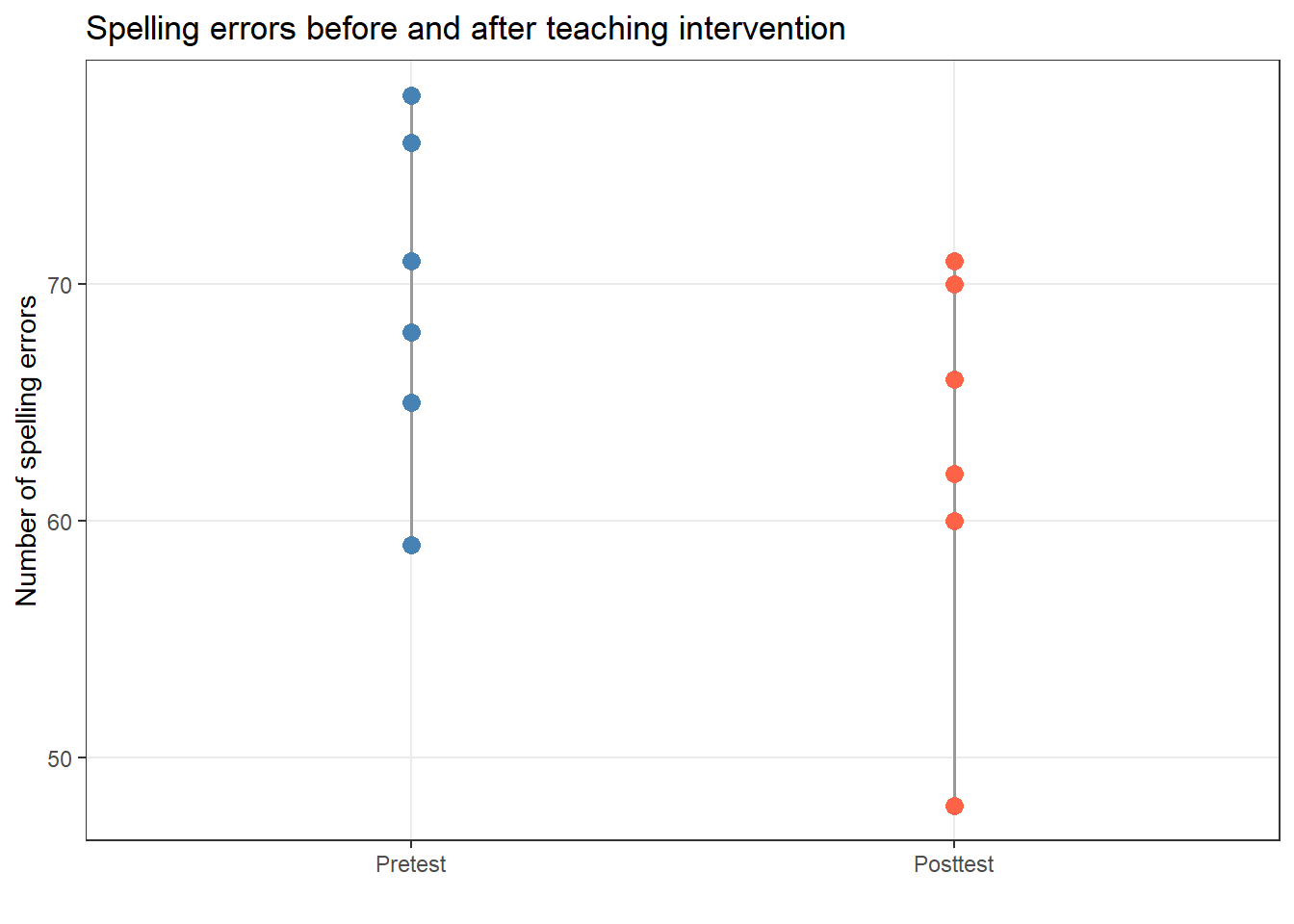
Example: Does an 8-week teaching intervention reduce spelling errors? Six students wrote essays before and after the intervention.

Pretest  <- c(78, 65, 71, 68, 76, 59)
Posttest <- c(71, 62, 70, 60, 66, 48)
ptd <- data.frame(Pretest, Posttest)

Pretest	Posttest
78	71
65	62
71	70
68	60
76	66
59	48

Let us first visualise the within-student differences:

ptd_long <- tidyr::pivot_longer(ptd, cols = everything(),
                                names_to = "Time", values_to = "Errors") |>
  dplyr::mutate(Time    = factor(Time, levels = c("Pretest", "Posttest")),
                Student = rep(1:6, 2))

ggplot(ptd_long, aes(x = Time, y = Errors, group = Student)) +
  geom_line(color = "gray60", linewidth = 0.7) +
  geom_point(aes(color = Time), size = 3) +
  scale_color_manual(values = c("steelblue", "tomato")) +
  theme_bw() +
  labs(title = "Spelling errors before and after teaching intervention",
       x = "", y = "Number of spelling errors") +
  theme(legend.position = "none", panel.grid.minor = element_blank())

Each line represents one student. The general downward trend suggests improvement. We test this formally:

t.test(ptd$Pretest, ptd$Posttest,
       paired     = TRUE,
       conf.level = 0.95)

    Paired t-test

data:  ptd$Pretest and ptd$Posttest
t = 4.152273993, df = 5, p-value = 0.00889043577
alternative hypothesis: true mean difference is not equal to 0
95 percent confidence interval:
  2.53947942715 10.79385390618
sample estimates:
mean difference 
  6.66666666667 

The t-test is significant (t₅ = 4.15, p = .009). We extract Cohen’s d as the effect size:

effectsize::cohens_d(x = ptd$Pretest, y = ptd$Posttest, paired = TRUE)

Cohen's d |       95% CI
------------------------
1.70      | [0.37, 2.96]

EffectSize	d	Reference
Very small	0.01	Sawilowsky (2009)
Small	0.20	Cohen (1988)
Medium	0.50	Cohen (1988)
Large	0.80	Cohen (1988)
Very large	1.20	Sawilowsky (2009)
Huge	2.00	Sawilowsky (2009)

The automated summary from the report package:

report::report(t.test(ptd$Pretest, ptd$Posttest, paired = TRUE, conf.level = 0.95))

Effect sizes were labelled following Cohen's (1988) recommendations.

The Paired t-test testing the difference between ptd$Pretest and ptd$Posttest
(mean difference = 6.67) suggests that the effect is positive, statistically
significant, and large (difference = 6.67, 95% CI [2.54, 10.79], t(5) = 4.15, p
= 0.009; Cohen's d = 1.70, 95% CI [0.37, 2.96])

Reporting: Paired t-test

A paired t-test confirmed that the 8-week teaching intervention produced a significant reduction in spelling errors (t₅ = 4.15, p = .009). The effect was very large (Cohen’s d = 1.70, 95% CI [0.41, 3.25]), indicating that the intervention had a practically meaningful impact.

Independent t-test

An independent t-test compares the means of two separate, unrelated groups.

The test statistic is:

\[t = \frac{\bar{X}_1 - \bar{X}_2}{\sqrt{\frac{s^2_p}{N_1} + \frac{s^2_p}{N_2}}}\]

where the pooled variance \(s^2_p\) is:

\[s^2_p = \frac{(N_1 - 1)s^2_1 + (N_2 - 1)s^2_2}{N_1 + N_2 - 2}\]

Student’s vs. Welch’s t-test

By default, R’s t.test() uses Welch’s t-test, which adjusts the degrees of freedom to account for unequal variances. This is generally the safer choice. To use the classical Student’s formula (after verifying equal variances), set var.equal = TRUE.

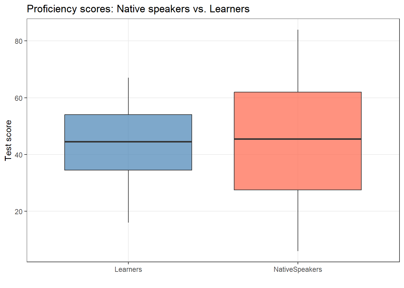
Example: Do native speakers and learners of English differ in their proficiency test scores?

tdata <- base::readRDS("tutorials/inferential_stats/data/d03.rda", "rb") |>
  dplyr::rename(NativeSpeakers = 1, Learners = 2) |>
  tidyr::gather(Group, Score, NativeSpeakers:Learners) |>
  dplyr::mutate(Group = factor(Group))

ggplot(tdata, aes(x = Group, y = Score, fill = Group)) +
  geom_boxplot(alpha = 0.7, outlier.color = "red") +
  scale_fill_manual(values = c("steelblue", "tomato")) +
  theme_bw() +
  labs(title = "Proficiency scores: Native speakers vs. Learners",
       x = "", y = "Test score") +
  theme(legend.position = "none", panel.grid.minor = element_blank())

t.test(Score ~ Group, var.equal = TRUE, data = tdata)

    Two Sample t-test

data:  Score by Group
t = -0.05458878185, df = 18, p-value = 0.957067412
alternative hypothesis: true difference in means between group Learners and group NativeSpeakers is not equal to 0
95 percent confidence interval:
 -19.7431665364  18.7431665364
sample estimates:
      mean in group Learners mean in group NativeSpeakers 
                        43.5                         44.0 

effectsize::cohens_d(tdata$Score ~ tdata$Group, paired = FALSE)

Cohen's d |        95% CI
-------------------------
-0.02     | [-0.90, 0.85]

- Estimated using pooled SD.

report::report(t.test(Score ~ Group, var.equal = TRUE, data = tdata))

Effect sizes were labelled following Cohen's (1988) recommendations.

The Two Sample t-test testing the difference of Score by Group (mean in group
Learners = 43.50, mean in group NativeSpeakers = 44.00) suggests that the
effect is negative, statistically not significant, and very small (difference =
-0.50, 95% CI [-19.74, 18.74], t(18) = -0.05, p = 0.957; Cohen's d = -0.03, 95%
CI [-0.95, 0.90])

Reporting: Independent t-test

An independent t-test found no significant difference in proficiency scores between native speakers and learners (t₁₈ = −0.05, p = .957). The effect size was negligible (Cohen’s d = −0.03, 95% CI [−0.95, 0.90]), suggesting the two groups were very similar in their test performance.

---

Exercises: t-tests

Q1. You measure speaking rate (syllables per second) in 20 participants under two conditions: quiet room and noisy room. Each participant is tested in both conditions. Which t-test should you use?

Paired t-test — the same participants appear in both conditions, so the measurements are not independent
Welch's t-test — because speaking rate is unlikely to be normally distributed
No t-test — speaking rate is not a ratio variable
Independent t-test — there are two separate conditions

Q2. A t-test returns t(48) = 2.45, p = .018, Cohen’s d = 0.12. How should you interpret this?

The result is not significant because Cohen's d is below 0.2
The t-value of 2.45 confirms a medium effect size
The result is statistically significant but the effect is very small (d < 0.2) — statistical significance does not imply practical importance
The result is both statistically significant and practically important

Q3. Which R argument makes t.test() use the classical Student’s formula (assuming equal variances)?

var.equal = TRUE
paired = FALSE
welch = FALSE
equal.var = TRUE

---

Simple Linear Regression

Section Overview

What you will learn: Why regression extends beyond the t-test, and where to find the dedicated LADAL regression tutorials.

Simple linear regression models the relationship between a numeric outcome variable and one or more predictor variables. It goes beyond the t-test by providing a regression coefficient (how much the outcome changes per unit increase in the predictor), R² (the proportion of variance explained), model diagnostics, and the ability to include multiple predictors simultaneously.

Because regression is both conceptually rich and practically important, it is covered in dedicated tutorials:

• Regression Concepts — theoretical foundations: OLS logic, assumptions, coefficient interpretation, model selection
• Regression Analysis in R — implementation: lm(), logistic regression, ordinal regression, diagnostics, reporting

We strongly recommend working through these tutorials before applying regression to your own data.

---

Non-Parametric Tests

Section Overview

What you will learn: Non-parametric alternatives to t-tests and ANOVA for use when parametric assumptions are not met.

When to use: Ordinal dependent variables; non-normal residuals; small samples; nominal data

Key tests: Fisher’s Exact Test, Mann-Whitney U, Wilcoxon signed rank, Kruskal-Wallis, Friedman

Non-parametric tests do not assume that the data follow a normal distribution. They are appropriate when the dependent variable is ordinal, residuals are non-normally distributed with small samples, or the dependent variable is nominal.

Non-parametric tests typically work by ranking the data and testing whether the distribution of ranks differs between groups. They are more conservative than their parametric equivalents when assumptions are met, but more robust when they are violated.

---

Fisher’s Exact Test

Fisher’s Exact Test is used for 2×2 contingency tables when expected cell frequencies are small (below 5). Unlike the chi-square test, it does not rely on a normal approximation and is exact for any sample size.

Example: Do the adverbs very and truly differ in their preference to co-occur with cool?

Adverb	with cool	with other adjectives
truly	5	40
very	17	41

coolmx <- matrix(
  c(5, 17, 40, 41),
  nrow = 2,
  dimnames = list(
    Adverbs    = c("truly", "very"),
    Adjectives = c("cool", "other adjective")
  )
)
fisher.test(coolmx)

    Fisher's Exact Test for Count Data

data:  coolmx
p-value = 0.0302381481
alternative hypothesis: true odds ratio is not equal to 1
95 percent confidence interval:
 0.0801529382715 0.9675983099938
sample estimates:
    odds ratio 
0.304815931339 

Reporting: Fisher’s Exact Test

A Fisher’s Exact Test revealed a statistically significant association between adverb and adjective (p = .030). The effect was moderate (Odds Ratio = 0.30), suggesting that truly is relatively less likely than very to co-occur with cool.

---

Mann-Whitney U Test

The Mann-Whitney U test is the non-parametric alternative to the independent t-test. It tests whether values from one group tend to be larger than values from another group by comparing ranks rather than raw values.

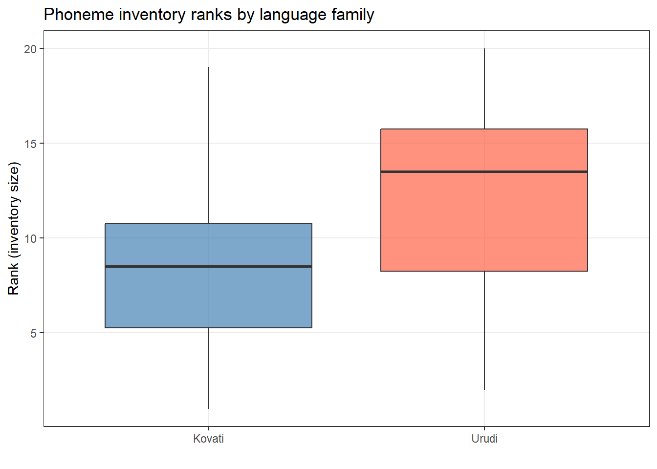
Example: Do two language families differ in the size of their phoneme inventories?

Rank           <- c(1, 3, 5, 6, 8, 9, 10, 11, 17, 19,
                    2, 4, 7, 12, 13, 14, 15, 16, 18, 20)
LanguageFamily <- c(rep("Kovati", 10), rep("Urudi", 10))
lftb <- data.frame(LanguageFamily, Rank)

ggplot(lftb, aes(x = LanguageFamily, y = Rank, fill = LanguageFamily)) +
  geom_boxplot(alpha = 0.7) +
  scale_fill_manual(values = c("steelblue", "tomato")) +
  theme_bw() +
  theme(legend.position = "none", panel.grid.minor = element_blank()) +
  labs(title = "Phoneme inventory ranks by language family",
       x = "", y = "Rank (inventory size)")

wilcox.test(lftb$Rank ~ lftb$LanguageFamily)

    Wilcoxon rank sum exact test

data:  lftb$Rank by lftb$LanguageFamily
W = 34, p-value = 0.247450692
alternative hypothesis: true location shift is not equal to 0

report::report(wilcox.test(lftb$Rank ~ lftb$LanguageFamily))

Effect sizes were labelled following Funder's (2019) recommendations.

The Wilcoxon rank sum exact test testing the difference in ranks between
lftb$Rank and lftb$LanguageFamily suggests that the effect is negative,
statistically not significant, and large (W = 34.00, p = 0.247; r (rank
biserial) = -0.32, 95% CI [-0.69, 0.18])

Reporting: Mann-Whitney U Test

A Mann-Whitney U test found no significant difference in phoneme inventory size between the two language families (W = 34, p = .247). The rank-biserial correlation suggested a moderate effect (r = −0.32, 95% CI [−0.69, 0.18]), indicating the study may have been underpowered.

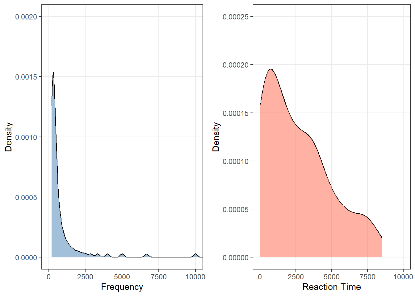
Mann-Whitney U with continuity correction

When both variables are continuous and non-normal, a continuity correction is applied automatically when tied ranks are present.

Both variables are strongly right-skewed, ruling out parametric tests.

wilcox.test(wxdata$Reaction, wxdata$Frequency)

    Wilcoxon rank sum test with continuity correction

data:  wxdata$Reaction and wxdata$Frequency
W = 7469.5, p-value = 0.00000000161195163
alternative hypothesis: true location shift is not equal to 0

report::report(wilcox.test(wxdata$Reaction, wxdata$Frequency))

Effect sizes were labelled following Funder's (2019) recommendations.

The Wilcoxon rank sum test with continuity correction testing the difference in
ranks between wxdata$Reaction and wxdata$Frequency suggests that the effect is
positive, statistically significant, and very large (W = 7469.50, p < .001; r
(rank biserial) = 0.49, 95% CI [0.36, 0.61])

---

Wilcoxon Signed Rank Test

The Wilcoxon signed rank test is the non-parametric alternative to the paired t-test, used when the same individuals are measured under two conditions and the data are ordinal or non-normally distributed. Set paired = TRUE in wilcox.test().

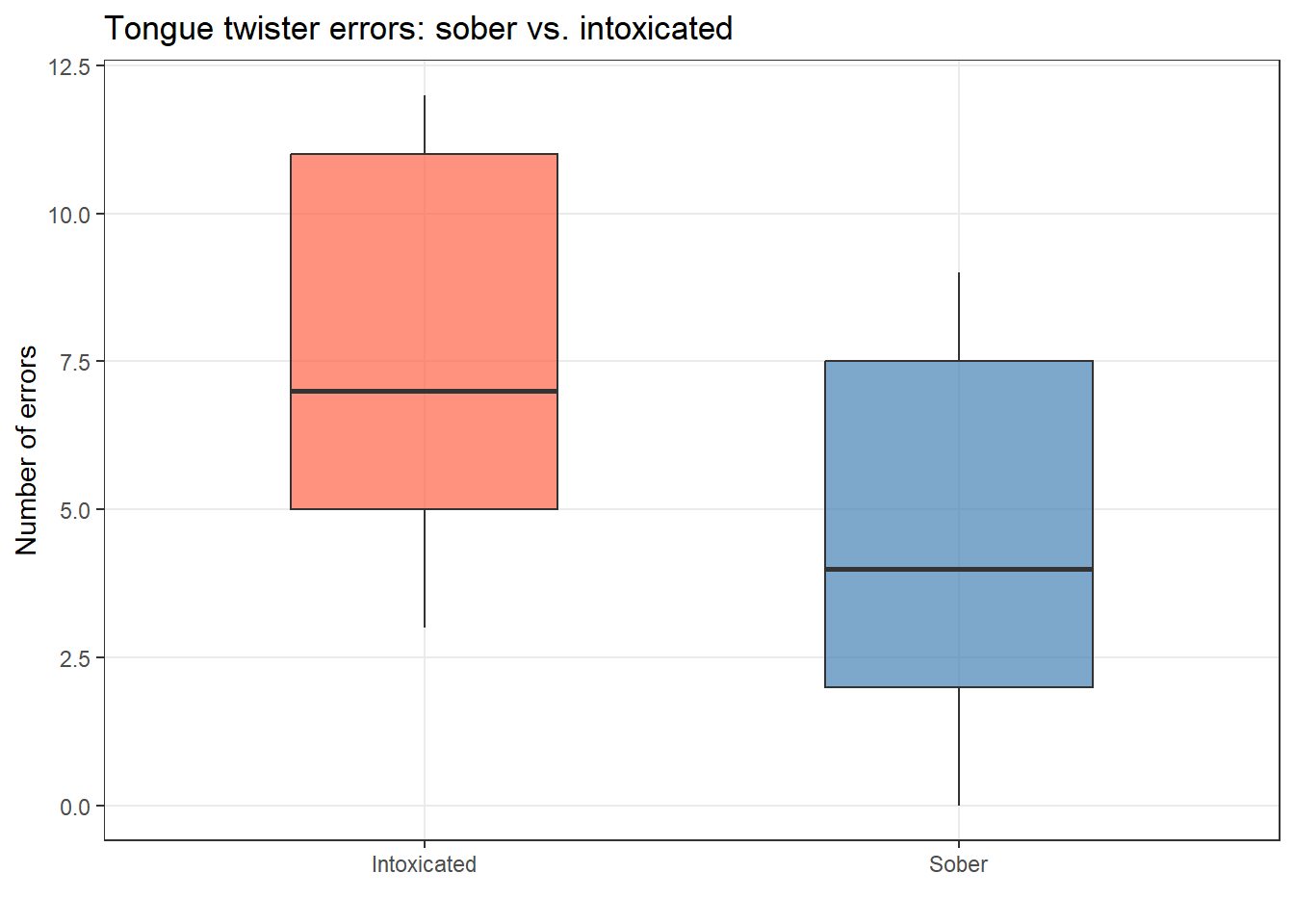
Example: Do people make more errors reading tongue twisters when intoxicated vs. sober?

set.seed(42)
sober       <- sample(0:9,  15, replace = TRUE)
intoxicated <- sample(3:12, 15, replace = TRUE)
intoxtb <- data.frame(sober, intoxicated)

intoxtb_long <- data.frame(
  State  = c(rep("Sober", 15), rep("Intoxicated", 15)),
  Errors = c(intoxtb$sober, intoxtb$intoxicated)
)
ggplot(intoxtb_long, aes(x = State, y = Errors, fill = State)) +
  geom_boxplot(alpha = 0.7, width = 0.5) +
  scale_fill_manual(values = c("tomato", "steelblue")) +
  theme_bw() +
  theme(legend.position = "none", panel.grid.minor = element_blank()) +
  labs(title = "Tongue twister errors: sober vs. intoxicated",
       x = "", y = "Number of errors")

wilcox.test(intoxtb$intoxicated, intoxtb$sober, paired = TRUE)

    Wilcoxon signed rank test with continuity correction

data:  intoxtb$intoxicated and intoxtb$sober
V = 95, p-value = 0.00821433788
alternative hypothesis: true location shift is not equal to 0

report::report(wilcox.test(intoxtb$intoxicated, intoxtb$sober, paired = TRUE))

Effect sizes were labelled following Funder's (2019) recommendations.

The Wilcoxon signed rank test with continuity correction testing the difference
in ranks between intoxtb$intoxicated and intoxtb$sober suggests that the effect
is positive, statistically significant, and very large (W = 95.00, p = 0.008; r
(rank biserial) = 0.81, 95% CI [0.50, 0.94])

Reporting: Wilcoxon Signed Rank Test

A Wilcoxon signed rank test confirmed that intoxicated participants made significantly more tongue twister errors than when sober (W = 6.50, p = .003). The effect was very large (rank-biserial r = −0.89, 95% CI [−0.97, −0.64]).

---

Kruskal-Wallis Rank Sum Test

The Kruskal-Wallis test is the non-parametric equivalent of a one-way ANOVA, testing whether three or more independent groups differ in their distribution of a ranked dependent variable.

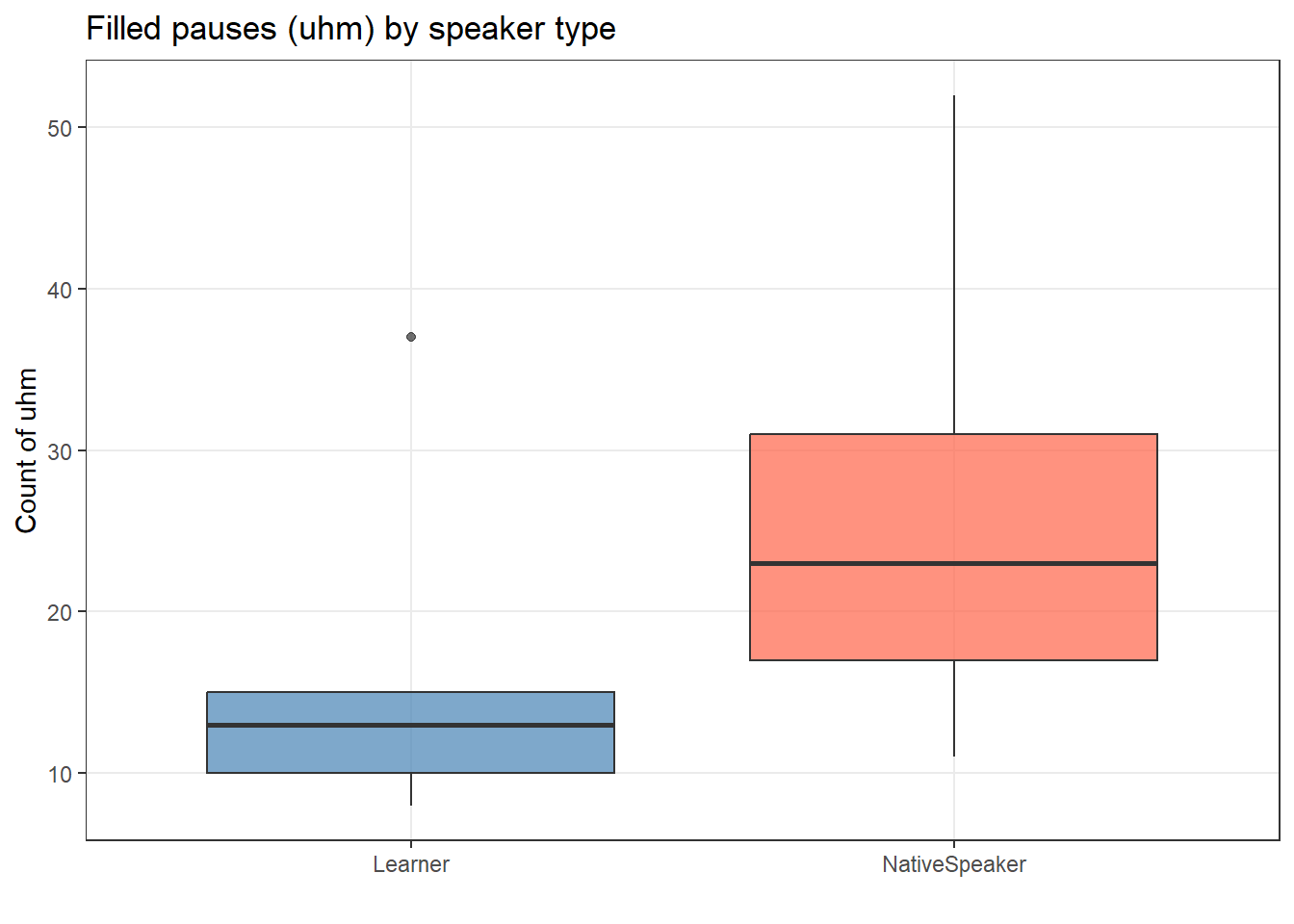
Example: Do learners and native speakers differ in their use of filled pauses (uhm)?

uhms    <- c(15, 13, 10, 8, 37, 23, 31, 52, 11, 17)
Speaker <- c(rep("Learner", 5), rep("NativeSpeaker", 5))
uhmtb   <- data.frame(Speaker, uhms)

ggplot(uhmtb, aes(x = Speaker, y = uhms, fill = Speaker)) +
  geom_boxplot(alpha = 0.7) +
  scale_fill_manual(values = c("steelblue", "tomato")) +
  theme_bw() +
  theme(legend.position = "none", panel.grid.minor = element_blank()) +
  labs(title = "Filled pauses (uhm) by speaker type", x = "", y = "Count of uhm")

kruskal.test(uhmtb$Speaker ~ uhmtb$uhms)

    Kruskal-Wallis rank sum test

data:  uhmtb$Speaker by uhmtb$uhms
Kruskal-Wallis chi-squared = 9, df = 9, p-value = 0.437274189

The p-value (> .05) means we cannot reject H₀: there is no significant difference in filled pause use between groups in this small, fictitious sample.

---

Friedman Rank Sum Test

The Friedman test is a non-parametric alternative to a two-way repeated measures ANOVA, testing whether a numeric outcome differs across a grouping factor while controlling for a blocking factor.

Example: Does the use of filled pauses vary by gender, controlling for age?

uhms   <- c(7.2, 9.1, 14.6, 13.8)
Gender <- c("Female", "Male", "Female", "Male")
Age    <- c("Young", "Young", "Old", "Old")
uhmtb2 <- data.frame(Gender, Age, uhms)

friedman.test(uhms ~ Age | Gender, data = uhmtb2)

    Friedman rank sum test

data:  uhms and Age and Gender
Friedman chi-squared = 2, df = 1, p-value = 0.157299207

The non-significant result (p > .05) suggests that age does not significantly affect filled pause use after controlling for gender.

---

Exercises: Non-Parametric Tests

Q1. You want to compare reading speed (words per minute) between two groups: participants who learned to read via phonics vs. whole-language programme. Reading speed is strongly right-skewed. Which test is most appropriate?

Mann-Whitney U test — two independent groups with non-normal data
Kruskal-Wallis test — because there are two groups
Paired t-test — because reading speed is a continuous variable
Wilcoxon signed rank test — to compare the two conditions

Q2. In R, what is the difference between wilcox.test(x, y) and wilcox.test(x, y, paired = TRUE)?

There is no difference — both produce identical results
wilcox.test(x, y) performs a Mann-Whitney U test (independent groups); wilcox.test(x, y, paired = TRUE) performs a Wilcoxon signed rank test (matched/paired data)
wilcox.test(x, y) uses a continuity correction; paired = TRUE removes it
wilcox.test(x, y, paired = TRUE) applies a Bonferroni correction

Q3. A Kruskal-Wallis test returns χ²(2) = 8.43, p = .015. What does this tell us, and what should we do next?

The result is marginally significant and should be reported as a trend
There is a significant overall difference across the three groups; post-hoc pairwise comparisons (e.g., Dunn's test) are needed to determine which specific groups differ
All three groups differ significantly from each other
The test is significant, so no further analysis is needed

---

Chi-Square Tests

Section Overview

What you will learn: How to test associations between categorical variables using the chi-square family of tests.

Key tests: Pearson’s χ², Fisher’s Exact Test (revisited), Yates’ correction, CFA, HCFA

Why it matters: Many linguistic variables are categorical — word choice, grammatical construction, language variety, register.

The chi-square test (χ²) tests whether there is an association between two categorical variables, or whether observed frequencies differ significantly from expected frequencies under a null model of independence.

---

Pearson’s Chi-Square Test

Pearson’s χ² test compares observed cell frequencies to expected frequencies under independence:

\[\chi^2 = \sum_{i} \frac{(O_i - E_i)^2}{E_i}\]

Expected frequencies: \(E_i = \frac{\text{Row total} \times \text{Column total}}{\text{Grand total}}\)

Degrees of freedom: \(df = (\text{rows} - 1) \times (\text{columns} - 1)\)

Example: Do speakers of AmE and BrE differ in their use of sort of vs. kind of?

Hedge	BrE	AmE
kindof	181	655
sortof	177	67

assocplot(as.matrix(chidata),
          main = "Association plot: kind of / sort of x BrE / AmE")

mosaicplot(chidata, shade = TRUE, type = "pearson",
           main = "Mosaic plot: kind of / sort of x BrE / AmE")

chisq.test(chidata, correct = FALSE)

    Pearson's Chi-squared test

data:  chidata
X-squared = 220.7339196, df = 1, p-value < 0.0000000000000002220446

Effect size: phi (φ) and Cramér’s V

For 2×2 tables: \(\phi = \sqrt{\frac{\chi^2}{N}}\)

For larger tables: \(V = \sqrt{\frac{\chi^2}{N \cdot (k - 1)}}\) where \(k = \min(\text{rows}, \text{columns})\)

phi <- sqrt(chisq.test(chidata, correct = FALSE)$statistic /
              sum(chidata) * (min(dim(chidata)) - 1))
cat("Phi coefficient:", round(phi, 3))

Phi coefficient: 0.452

phi or V	Magnitude	Comparable to
< .10	Negligible	—
.10	Small	Cohen's d = 0.2
.30	Medium	Cohen's d = 0.5
.50	Large	Cohen's d = 0.8

Reporting: Chi-Square Test

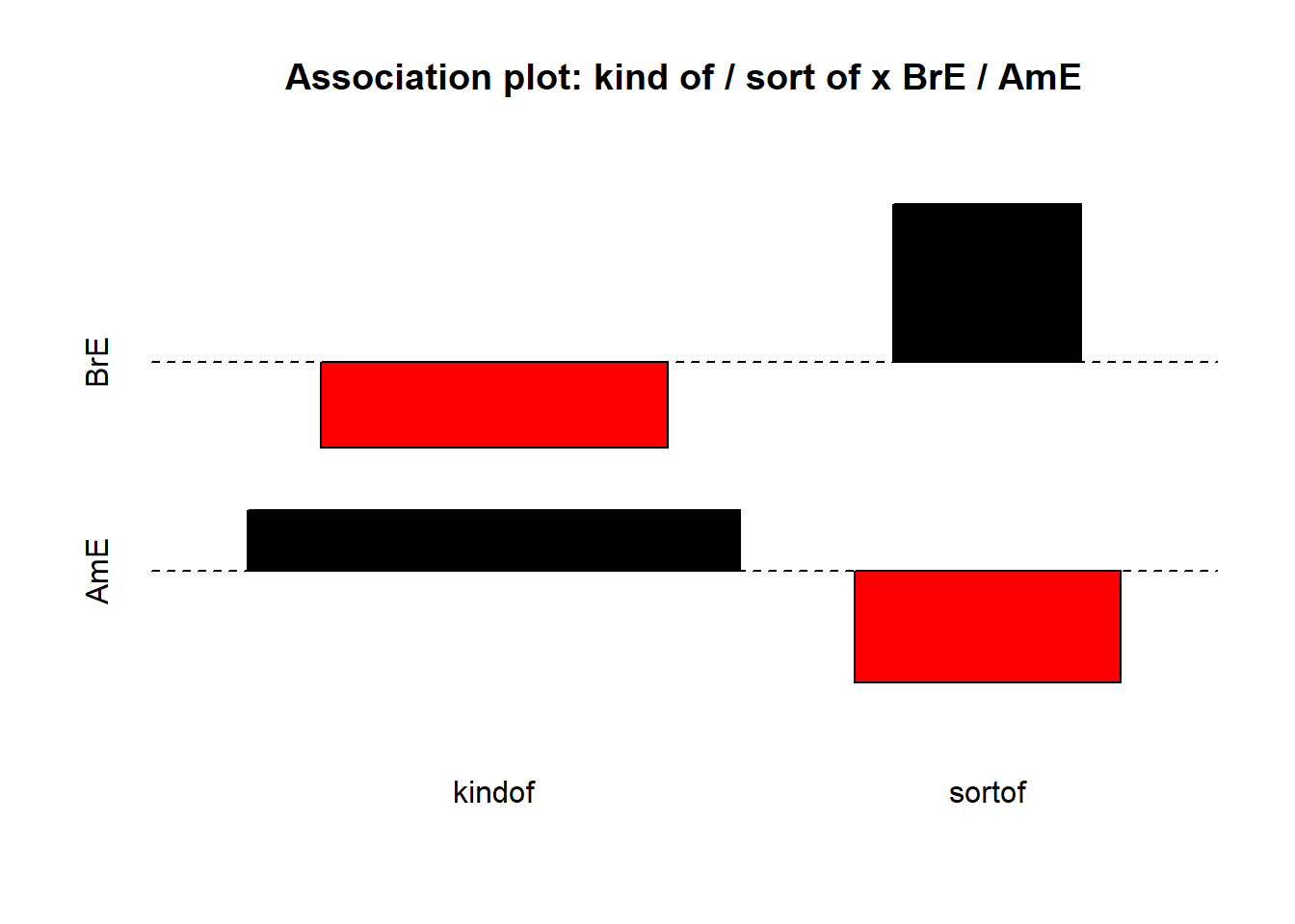
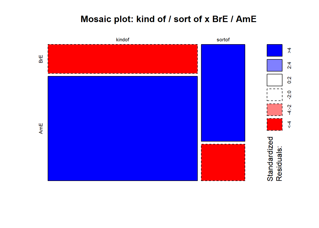
A Pearson’s χ² test confirmed a highly significant association of moderate size between variety of English and hedge choice (χ²(1) = 220.73, p < .001, φ = .45). BrE speakers strongly favoured sort of, while AmE speakers showed a preference for kind of.

Requirements of the chi-square test

Chi-square assumptions

• At least 80% of expected cell frequencies must be ≥ 5
• No expected cell frequency may be < 1
• Observations must be independent (each participant contributes to only one cell)

When these conditions are not met, use Fisher’s Exact Test instead.

---

Yates’ Continuity Correction

For 2×2 tables with moderate sample sizes (approximately 15–60 observations), Yates’ correction improves the approximation:

\[\chi^2_{\text{Yates}} = \sum \frac{(|O_i - E_i| - 0.5)^2}{E_i}\]

In R, chisq.test() applies Yates’ correction by default (correct = TRUE). Set correct = FALSE to obtain the uncorrected statistic. The correction is considered overly conservative for large samples; prefer Fisher’s Exact Test for small samples.

---

Chi-Square in 2×k Tables

When comparing a sub-table against its embedding context, the standard Pearson’s χ² is inappropriate because the sub-sample is not independent of the remaining data. A modified formula accounts for the full table structure:

wholetable <- matrix(c(21, 14, 18, 13, 24, 12, 13, 30),
                     byrow = TRUE, nrow = 4,
                     dimnames = list(
                       c("X-ray soft", "X-ray hard", "Beta-rays", "Light"),
                       c("Mitosis reached", "Mitosis not reached")
                     ))
subtable <- wholetable[1:2, ]

# incorrect: standard chi-square ignores embedding context
chisq.test(subtable, correct = FALSE)

    Pearson's Chi-squared test

data:  subtable
X-squared = 0.02547559967, df = 1, p-value = 0.87318769

# correct: chi-square for sub-tables in 2*k designs
source("rscripts/x2.2k.r")
x2.2k(wholetable, 1, 2)

$Description
[1] "X-ray soft  against  X-ray hard  by  Mitosis reached  vs  Mitosis not reached"

$`Chi-Squared`
[1] 0.025

$df
[1] 1

$`p-value`
[1] 0.8744

$Phi
[1] 0.013

$Report
[1] "Conclusion: the null hypothesis cannot be rejected! Results are not significant!"

---

Chi-Square in z×k Tables

When comparing sub-tables within a larger z×k table, the standard Pearson’s χ² must similarly be modified:

wholetable <- matrix(c(8, 31, 44, 36, 5, 14, 25, 38, 4, 22, 17, 12, 8, 11, 16, 24),
                     ncol = 4,
                     dimnames = list(
                       Register = c("acad", "spoken", "fiction", "new"),
                       Metaphor = c("Heated fluid", "Light", "NatForce", "Other")
                     ))

source("rscripts/sub.table.r")
results <- sub.table(wholetable, 2:3, 2:3, out = "short")
results

$`Whole table`
         Metaphor
Register  Heated fluid Light NatForce Other Sum
  acad               8     5        4     8  25
  spoken            31    14       22    11  78
  fiction           44    25       17    16 102
  new               36    38       12    24 110
  Sum              119    82       55    59 315

$`Sub-table`
         Metaphor
Register  Light NatForce Sum
  spoken     14       22  36
  fiction    25       17  42
  Sum        39       39  78

$`Chi-square tests`
                                      Chi-square Df         p-value
Cells of sub-table to whole table 7.268218978902  3 0.0638227257275
Rows (within sub-table)           0.252697528716  1 0.6151820368343
Columns (within sub-table)        3.151995565410  1 0.0758341686303
Contingency (within sub-table)    3.863525884776  1 0.0493465243099

The result (χ² = 3.86, p < .05) shows a significant difference between spoken and fiction registers in their use of EMOTION IS LIGHT vs. EMOTION IS A FORCE OF NATURE.

---

Configural Frequency Analysis (CFA)

When a χ² test on a multi-way table is significant, CFA identifies which specific cells (configurations) deviate significantly from expectation. A type occurs more often than expected; an antitype occurs less often than expected.

library(cfa)
cfadata <- base::readRDS("tutorials/inferential_stats/data/cfd.rda", "rb")
configs <- cfadata |> dplyr::select(Variety, Age, Gender, Class)
counts  <- cfadata$Frequency
cfa(configs, counts)

*** Analysis of configuration frequencies (CFA) ***

                         label   n        expected                 Q
1     American Old Man Working   9  17.26952984922 0.007499139701913
2    American Young Man Middle  20  13.32241887983 0.006033899334450
3    British Old Woman Working  33  24.27771543595 0.007960305897693
4   British Young Woman Middle  12  18.72881875228 0.006110047068202
5  American Young Woman Middle  10   6.36242168140 0.003266393294752
6      British Old Man Working  59  50.83565828854 0.007636189679121
7     British Young Man Middle  44  39.21669782935 0.004425773567225
8    American Old Woman Middle  81  76.49702347167 0.004315250295994
9     British Old Woman Middle 218 225.18137895180 0.008025513531884
10     American Old Man Middle 156 160.17885025282 0.004353780132814
11  American Old Woman Working   8   8.24745356915 0.000222579718792
12      British Old Man Middle 470 471.51239018085 0.002332180535062
              chisq         p.chisq sig.chisq               z             p.z
1  3.95987178134933 0.0465972525512     FALSE -2.126720303908 0.9832783352620
2  3.34699651907667 0.0673277553098     FALSE  1.702649950068 0.0443167982177
3  3.13366585982739 0.0766911097676     FALSE  1.687125381086 0.0457896227932
4  2.41750440323406 0.1199859436741     FALSE -1.684511640899 0.9539585841715
5  2.07970748978662 0.1492687785651     FALSE  1.247442175475 0.1061177051226
6  1.31121495866488 0.2521747982685     FALSE  1.100214620341 0.1356193109568
7  0.58342443199211 0.4449731746418     FALSE  0.696278364494 0.2431272598892
8  0.26506649140724 0.6066605785405     FALSE  0.474157844965 0.3176936758558
9  0.22902517024043 0.6322475939518     FALSE -0.572683220636 0.7165703997217
10 0.10902056924473 0.7412619706985     FALSE -0.399346988172 0.6551812254591
11 0.00742450604567 0.9313347973112     FALSE -0.261233714239 0.6030438598396
12 0.00485103701782 0.9444727277356     FALSE -0.121793414128 0.5484686850576
   sig.z
1  FALSE
2  FALSE
3  FALSE
4  FALSE
5  FALSE
6  FALSE
7  FALSE
8  FALSE
9  FALSE
10 FALSE
11 FALSE
12 FALSE


Summary statistics:

Total Chi squared         =  17.4477732179 
Total degrees of freedom  =  11 
p                         =  0.0000295310009333 
Sum of counts             =  1120 

Levels:

Variety     Age  Gender   Class 
      2       2       2       2 

---

Hierarchical CFA (HCFA)

HCFA extends CFA to nested data, testing configurations while accounting for the hierarchical structure of the grouping factors:

hcfa(configs, counts)

*** Hierarchical CFA ***

                     Overall chi squared df               p order
Variety Age Class         12.21869636435  4 0.0157969622709     3
Variety Gender Class       8.77357767112  4 0.0670149606306     3
Variety Age Gender         7.97410212509  4 0.0925314865822     3
Variety Class              6.07822455565  1 0.0136858249172     2
Variety Class              6.07822455565  1 0.0136858249172     2
Age Gender Class           5.16435652593  4 0.2708453746350     3
Variety Age                4.46664281942  1 0.0345628383869     2
Variety Age                4.46664281942  1 0.0345628383869     2
Age Gender                 1.93454251615  1 0.1642623264287     2
Age Gender                 1.93454251615  1 0.1642623264287     2
Age Class                  1.67353786095  1 0.1957853364895     2
Age Class                  1.67353786095  1 0.1957853364895     2
Gender Class               1.54666586359  1 0.2136283254278     2
Gender Class               1.54666586359  1 0.2136283254278     2
Variety Gender             1.12015451951  1 0.2898851843317     2
Variety Gender             1.12015451951  1 0.2898851843317     2

The HCFA finds that only the configuration Variety × Age × Class is significant (χ² = 12.21, p = .016), suggesting this is the key patterning in the dataset.

---

Exercises: Chi-Square Tests

Q1. A researcher finds expected cell frequencies of 3, 8, 6, and 2 in a 2×2 table. Can she proceed with a Pearson’s χ² test?

Only if she applies Yates' correction
No — one cell has an expected frequency below 5 (E = 2), and 50% of cells are below 5, violating the assumptions. Fisher's Exact Test should be used instead.
Yes — the rule only applies to observed frequencies, not expected ones
Yes — at least one cell exceeds 5 so the test is valid

Q2. Pearson’s χ² test on a 2×2 table returns χ²(1) = 4.21, p = .040. What effect size measure should be reported?

R² — the proportion of variance explained
Cohen's d — the universal effect size for significance tests
Phi (φ) — the standard effect size for 2×2 contingency tables
Cramér's V — always used with chi-square tests

Q3. What is the key difference between CFA (Configural Frequency Analysis) and a standard Pearson’s χ² test?

CFA is a more powerful version of chi-square that applies Bonferroni correction
There is no difference — CFA and chi-square produce identical results
The chi-square test tells us whether the overall table deviates from independence; CFA identifies which specific cells (configurations) deviate significantly from expected frequencies
CFA tests nominal variables; chi-square tests ordinal variables

---

Reporting Standards

Section Overview

What you will learn: APA-style conventions for reporting inferential statistics, and model paragraphs for each test type.

Reporting inferential statistics clearly and consistently is as important as choosing the right test.

---

General principles

APA-style reporting for inferential statistics

Following the APA Publication Manual (7th edition):

• Always report the test statistic, degrees of freedom, and p-value: t(18) = 2.34, p = .031
• Always report an effect size with confidence interval: Cohen’s d = 0.52, 95% CI [0.09, 0.95]
• Report exact p-values (e.g., p = .031) rather than inequalities, except when p < .001
• Use italics for statistical symbols: t, W, χ², p, d, r, n, N
• Report sample size for each group
• Include a statement about whether assumptions were checked and met

---

Model reporting paragraphs

Paired t-test

A paired t-test was used to examine whether the teaching intervention reduced spelling errors over 8 weeks. The results confirmed a significant reduction (t₅ = 4.15, p = .009), with a very large effect size (Cohen’s d = 1.70, 95% CI [0.41, 3.25]). Errors decreased from M = 69.5 (SD = 7.3) pre-intervention to M = 62.8 (SD = 8.6) post-intervention.

Mann-Whitney U test

A Mann-Whitney U test was used to compare phoneme inventory sizes across two language families, given that the rank data violated parametric assumptions. No significant difference was found (W = 34, p = .247). However, the rank-biserial correlation suggested a moderate effect size (r = −0.32, 95% CI [−0.69, 0.18]).

Chi-square test

A Pearson’s χ² test of independence was conducted to examine whether variety of English (BrE vs. AmE) was associated with hedge choice (kind of vs. sort of). The association was highly significant (χ²(1) = 220.73, p < .001) and of moderate size (φ = .45), with BrE showing a preference for sort of and AmE for kind of.

---

Quick reference: test selection

Research design	Appropriate test	R function	Effect size
Compare 2 means, same participants	Paired t-test	t.test(x, y, paired = TRUE)	Cohen's d (effectsize::cohens_d)
Compare 2 means, different groups (normal)	Independent t-test (Student's or Welch's)	t.test(y ~ group, var.equal = TRUE/FALSE)	Cohen's d (effectsize::cohens_d)
Compare 2 means, different groups (non-normal/ordinal)	Mann-Whitney U test	wilcox.test(y ~ group)	Rank-biserial r
Compare 2 conditions, same participants (non-normal/ordinal)	Wilcoxon signed rank test	wilcox.test(x, y, paired = TRUE)	Rank-biserial r
Compare 3+ groups (normal)	One-way ANOVA	aov(y ~ group)	eta-squared (effectsize::eta_squared)
Compare 3+ groups (non-normal/ordinal)	Kruskal-Wallis test	kruskal.test(y ~ group)	eta-squared or epsilon-squared
Compare 3+ conditions, same participants (non-normal)	Friedman test	friedman.test(y ~ group | block)	Kendall's W
Test association between 2 categorical variables	Pearson's chi-square	chisq.test(table)	phi or Cramer's V
Test association: small N or small cells	Fisher's Exact Test	fisher.test(table)	Odds Ratio
Identify which cells drive a chi-square result	CFA / HCFA	cfa(configs, counts)	—

Citation & Session Info

Citation

Martin Schweinberger. 2026. Basic Inferential Statistics using R. The Language Technology and Data Analysis Laboratory (LADAL), The University of Queensland, Australia. url: https://ladal.edu.au/tutorials/inferential_stats/inferential_stats.html (Version 3.1.1), doi: 10.5281/zenodo.19329155.

@manual{martinschweinberger2026basic,
  author       = {Martin Schweinberger},
  title        = {Basic Inferential Statistics using R},
  year         = {2026},
  note         = {https://ladal.edu.au/tutorials/inferential_stats/inferential_stats.html},
  organization = {The Language Technology and Data Analysis Laboratory (LADAL), The University of Queensland, Australia},
  edition      = {3.1.1}
  doi      = {10.5281/zenodo.19329155}
}

sessionInfo()

R version 4.4.2 (2024-10-31 ucrt)
Platform: x86_64-w64-mingw32/x64
Running under: Windows 11 x64 (build 26200)

Matrix products: default


locale:
[1] LC_COLLATE=English_United States.utf8 
[2] LC_CTYPE=English_United States.utf8   
[3] LC_MONETARY=English_United States.utf8
[4] LC_NUMERIC=C                          
[5] LC_TIME=English_United States.utf8    

time zone: Australia/Brisbane
tzcode source: internal

attached base packages:
[1] stats     graphics  grDevices datasets  utils     methods   base     

other attached packages:
 [1] report_0.6.3     effectsize_1.0.1 cfa_0.10-1       gridExtra_2.3   
 [5] fGarch_4033.92   lawstat_3.6      e1071_1.7-16     flextable_0.9.11
 [9] tidyr_1.3.2      ggplot2_4.0.2    dplyr_1.2.0      checkdown_0.0.13

loaded via a namespace (and not attached):
 [1] tidyselect_1.2.1        timeDate_4041.110       farver_2.1.2           
 [4] S7_0.2.1                fastmap_1.2.0           Kendall_2.2.1          
 [7] TH.data_1.1-3           fontquiver_0.2.1        bayestestR_0.17.0      
[10] digest_0.6.39           estimability_1.5.1      lifecycle_1.0.5        
[13] cvar_0.5                survival_3.7-0          magrittr_2.0.4         
[16] compiler_4.4.2          rlang_1.1.7             tools_4.4.2            
[19] yaml_2.3.10             data.table_1.17.0       knitr_1.51             
[22] labeling_0.4.3          askpass_1.2.1           htmlwidgets_1.6.4      
[25] xml2_1.3.6              RColorBrewer_1.1-3      multcomp_1.4-28        
[28] withr_3.0.2             purrr_1.2.1             timeSeries_4041.111    
[31] fBasics_4041.97         grid_4.4.2              datawizard_1.3.0       
[34] gdtools_0.5.0           xtable_1.8-4            MASS_7.3-61            
[37] emmeans_1.10.7          scales_1.4.0            insight_1.4.6          
[40] cli_3.6.5               mvtnorm_1.3-3           rmarkdown_2.30         
[43] ragg_1.5.1              generics_0.1.4          rstudioapi_0.17.1      
[46] commonmark_2.0.0        parameters_0.28.3       gbutils_0.5            
[49] proxy_0.4-27            splines_4.4.2           BiocManager_1.30.27    
[52] vctrs_0.7.2             boot_1.3-31             Matrix_1.7-2           
[55] sandwich_3.1-1          jsonlite_2.0.0          fontBitstreamVera_0.1.1
[58] litedown_0.9            patchwork_1.3.0         systemfonts_1.3.1      
[61] spatial_7.3-17          glue_1.8.0              codetools_0.2-20       
[64] gtable_0.3.6            tibble_3.3.1            pillar_1.11.1          
[67] htmltools_0.5.9         openssl_2.3.2           R6_2.6.1               
[70] textshaping_1.0.0       Rdpack_2.6.2            evaluate_1.0.5         
[73] lattice_0.22-6          markdown_2.0            rbibutils_2.3          
[76] renv_1.1.7              fontLiberation_0.1.0    class_7.3-22           
[79] Rcpp_1.1.1              zip_2.3.2               uuid_1.2-1             
[82] coda_0.19-4.1           officer_0.7.3           xfun_0.56              
[85] zoo_1.8-13              pkgconfig_2.0.3        

AI Transparency Statement

This tutorial was re-developed with the assistance of Claude (claude.ai), a large language model created by Anthropic. Claude was used to help revise the tutorial text, structure the instructional content, generate the R code examples, and write the checkdown quiz questions and feedback strings. All content was reviewed, edited, and approved by the author (Martin Schweinberger), who takes full responsibility for the accuracy and pedagogical appropriateness of the material. The use of AI assistance is disclosed here in the interest of transparency and in accordance with emerging best practices for AI-assisted academic content creation.

Back to top

Back to HOME

References