Analysing Learner Language with R

Great Court, The University of Queensland

Introduction

This tutorial introduces methods for analysing learner language — the written and spoken production of second language (L2) learners — using R. Learner language, also called interlanguage (Selinker, Swain, and Dumas 1975), is the systematic, rule-governed variety of language produced by a learner at a given point in their development. It differs from the target language in predictable ways that reflect the learner’s evolving grammatical and lexical knowledge, transfer from their first language (L1), and the specific instructional and communicative contexts they have encountered.

Corpus-based approaches to learner language — using collections of authentic learner texts known as learner corpora — have grown substantially since the 1990s (Granger 2009). They allow researchers to move beyond anecdotal observation and examine patterns of learner language systematically, at scale, and in comparison with the production of native or proficient speakers. The availability of well-annotated learner corpora and powerful R packages makes it possible to carry out many standard learner corpus analyses reproducibly, with relatively compact code.

This tutorial covers seven core analysis types, progressing from basic frequency-based methods to more linguistically sophisticated measures:

1. Concordancing — extracting and inspecting keyword-in-context (KWIC) lines
2. Frequency lists — ranking words by frequency, with and without stopwords
3. Sentence length — computing and comparing average sentence length across L1 groups
4. N-gram analysis — extracting bigrams and comparing their use between learners and L1 speakers
5. Collocations and collocation networks — identifying strongly co-occurring word pairs and visualising their relationships
6. Part-of-speech tagging and POS-sequence analysis — automatically tagging word classes and comparing grammatical patterns
7. Lexical diversity and readability — quantifying vocabulary richness and text complexity

Prerequisite Tutorials

Before working through this tutorial, please ensure you are familiar with:

• Getting Started with R and RStudio
• Loading, Saving, and Generating Data in R
• String Processing in R
• Regular Expressions in R
• Introduction to Text Analysis — Part 1

Learning Objectives

By the end of this tutorial you will be able to:

1. Load and inspect learner corpus data in R
2. Extract and sort KWIC concordances for words and phrases
3. Build and visualise frequency lists with and without stopwords
4. Compute normalised sentence length and compare it across L1 groups
5. Extract bigrams, normalise their frequencies, and test for significant learner–L1 differences using Fisher’s exact test with Bonferroni correction
6. Identify collocations using log-likelihood and visualise them as network graphs
7. POS-tag texts with udpipe and compare POS-sequence bigrams across groups
8. Calculate and compare multiple lexical diversity measures and Flesch readability scores
9. Detect and quantify spelling errors using hunspell
10. Interpret the results of these analyses in the context of second language acquisition research

Citation

Martin Schweinberger. 2026. Analysing Learner Language with R. The Language Technology and Data Analysis Laboratory (LADAL), The University of Queensland, Australia. url: https://ladal.edu.au/tutorials/learner_language/learner_language.html (Version 3.1.1), doi: 10.5281/zenodo.19332907.

Background: Learner Corpora

Section Overview

What you’ll learn: What learner corpora are, how they differ from native-speaker corpora, and an introduction to the two corpora used in this tutorial

A learner corpus is a principled, machine-readable collection of texts produced by L2 learners of a target language (Granger 2009). Learner corpora can contain written essays, spoken transcripts, or both. They are typically annotated with metadata about the learner — their L1 background, proficiency level, age, educational context, and the task type that elicited the text. This metadata makes it possible to compare production across L1 groups, proficiency levels, or task types, and to contrast learner production with that of native or expert speakers.

The analysis of learner corpora is central to the field of Learner Corpus Research (LCR), which applies corpus linguistic methods to questions in second language acquisition (SLA), language pedagogy, and language testing (Gilquin and Granger 2015). Common research questions include: Do learners over- or under-use certain words, constructions, or discourse markers relative to native speakers? Does lexical diversity increase with proficiency? Are spelling or grammatical error rates associated with L1 background? Do learners from different L1 backgrounds show distinct error profiles?

The ICLE and LOCNESS Corpora

This tutorial uses data from two well-known learner corpus resources:

ICLE — International Corpus of Learner English (Granger et al. 1993). ICLE contains argumentative essays written by advanced university-level EFL learners from 16 different L1 backgrounds. The essays in this tutorial are drawn from the German, Spanish, French, Italian, Polish, and Russian sub-corpora of ICLE.

LOCNESS — Louvain Corpus of Native English Essays (Granger, Sanders, and Connor 2005). LOCNESS contains essays written by native speakers of English, including British A-level students (the sub-corpus used here) and American university students. It provides the native-speaker baseline against which the ICLE learner data is compared.

Both corpora were compiled by the Centre for English Corpus Linguistics (CECL) at the Université catholique de Louvain, Belgium. The essays in this tutorial deal with the topic of transport, which is one of the prompt topics common to both ICLE and LOCNESS, enabling direct comparison between learner and native-speaker production on the same task.

Data Access

The ICLE and LOCNESS corpora are commercially licensed and cannot be distributed freely. In this tutorial we load pre-processed sub-samples hosted on the LADAL server, which is sufficient to follow all examples. If you wish to work with the full corpora, contact the CECL at UCLouvain.

---

Setup

Installing Packages

# Run once to install — comment out after installation
install.packages("quanteda")
install.packages("quanteda.textstats")
install.packages("quanteda.textplots")
install.packages("tidyverse")
install.packages("flextable")
install.packages("tidytext")
install.packages("udpipe")
install.packages("koRpus")
install.packages("stringi")
install.packages("hunspell")
install.packages("wordcloud2")
install.packages("tokenizers")
install.packages("checkdown")

Loading Packages

# Load at the start of every session
library(tidyverse)       # dplyr, ggplot2, stringr, tidyr
library(flextable)       # formatted display tables
library(tidytext)        # stop_words and tidy text utilities
library(udpipe)          # POS tagging
library(quanteda)        # corpus and KWIC infrastructure
library(quanteda.textstats)  # textstat_collocations, textstat_readability, textstat_lexdiv
library(quanteda.textplots)  # textplot_xray, textplot_network
library(koRpus)          # lexical diversity measures
library(stringi)         # string reversal for sorted concordances
library(hunspell)        # spell checking
library(wordcloud2)      # word cloud visualisation
library(tokenizers)      # sentence splitting and word counting
library(checkdown)       # interactive quiz questions

Loading the Data

We load seven essay files: two from LOCNESS (L1 British English, split across two files) and one each from six ICLE sub-corpora representing learners whose L1 is German, Spanish, French, Italian, Polish, or Russian.

# L1 English (LOCNESS — British A-level essays)
ns1 <- base::readRDS("tutorials/learner_language/data/LCorpus/ns1.rda", "rb")
ns2 <- base::readRDS("tutorials/learner_language/data/LCorpus/ns2.rda", "rb")

# L2 learners (ICLE sub-corpora)
es <- base::readRDS("tutorials/learner_language/data/LCorpus/es.rda", "rb")
de <- base::readRDS("tutorials/learner_language/data/LCorpus/de.rda", "rb")
fr <- base::readRDS("tutorials/learner_language/data/LCorpus/fr.rda", "rb")
it <- base::readRDS("tutorials/learner_language/data/LCorpus/it.rda", "rb")
pl <- base::readRDS("tutorials/learner_language/data/LCorpus/pl.rda", "rb")
ru <- base::readRDS("tutorials/learner_language/data/LCorpus/ru.rda", "rb")

Let us inspect the first few lines of the Russian learner data to see what the raw ICLE files look like:

ru %>%
  stringr::str_remove("<[A-Z]{4,4}.*") %>%   # remove ICLE file header tags
  na_if("") %>%
  na.omit() %>%
  head(5)

[1] "It is now a very wide spread opinion, that in the modern world there is no place for dreaming and imagination. Those who share this point of view usually say that at present we are so very much under the domination of science, industry, technology, ever-increasing tempo of our lives and so on, that neither dreaming nor imagination can possibly survive. Their usual argument is very simple - they suggest to their opponents to look at some samples of the modern art and to compare them to the masterpieces of the \"Old Masters\" of painting, music, literature."                                                                                                                                                                                                                                                                                                                                                                                                                                
[2] "As everything which is simple, the argument sounds very convincing. Of course, it is evident, that no modern writer, painter or musician can be compare to such names as Bach, Pushkin< Byron, Mozart, Rembrandt, Raffael et cetera. Modern pictures, in the majority of cases, seem to be merely repetitions or combinations of the images and methods of painting, invented very long before. The same is also true to modern verses, novels and songs."                                                                                                                                                                                                                                                                                                                                                                                                                                                                                                                                                        
[3] "But, I think, those, who put forward this argument, play - if I may put it like this - not fair game with their opponents, because such an approach presupposes the firm conviction, that dreaming and imagination can deal only with Arts, moreover, only with this \"well-established set\" of Arts, which includes music, painting, architecture, sculpture and literature. That is, a person, who follows the above-mentioned point of view tries to make his opponent take for granted the statement, the evidence of which is, to say the least, doubtful."                                                                                                                                                                                                                                                                                                                                                                                                                                                 
[4] "But actually, these are not only music, painting, writing which are the spheres to which one's dreaming and imagination can be applied. First of all, there are quite a few other \"arts\". Probably, these are not as well-established as those mentioned above, but they are also \"arts\", and besides, they flourish nowdays. Let us take cinema, for example. Originally, in the beginning of the century, it was only an entertainment for common people. But today we may already call it \"art\". Now it has a hundred years of its history, and we all know, that cinema is really able to create masterpieces. Our contemporaries, film-directors of this \"dominated by science, technology and industrialization\" century create at present films like \"The Good, The Bad, The Ugly\", \"8 ½\", \"Once Upon a Time in America\", \"Shining\" et cetera, which, perhaps, in the next century will be regarded by our descendants just like w regard Raffael's pictures or Shakespeare's sonnets now."
[5] "By the way, I can hardly observe any connection between the \"domination of science, technology and industrialization\" over our world and the decline of arts. There may be some other reasons for it, but niether science nor technology themselves. Moreover, scientific and technological progress may very often create new means and new ways to apply one's imagination and \"materialize\"one's dream. For example, the newest computer technology, I think, has already created a whole range of ways to apply one's imagination - the computer design, animation and plenty of other things - and still has a great capasity for developement."                                                                                                                                                                                                                                                                                                                                                         

The text is stored as a character vector where each element is typically a paragraph or a short passage. The <ICLE-...> header tag that appears at the top of each file encodes metadata (the learner’s L1, proficiency level, and essay topic); we strip this in subsequent processing steps.

We also create two combined objects — one pooling all L1 texts and one pooling all learner texts — which we will use throughout:

l1      <- c(ns1, ns2)                       # all native-speaker text
learner <- c(de, es, fr, it, pl, ru)         # all learner text

---

Concordancing

Section Overview

What you’ll learn: How to extract keyword-in-context (KWIC) concordances for individual words and phrases, how to sort them by preceding or following context, and how to visualise dispersion patterns across texts

Key function: quanteda::kwic()

Concordancing — the extraction of words or phrases from a corpus together with their surrounding context — is one of the most fundamental operations in corpus linguistics (Lindquist 2009). A keyword-in-context (KWIC) display places the search term in the centre of a fixed-width window of preceding and following tokens, making it easy to inspect how a word is actually used across many instances. KWIC concordances are useful for: verifying that a search pattern is returning the intended tokens; examining how learners use a specific word or construction compared to L1 speakers; extracting authentic examples for pedagogical or analytical purposes; and as a preliminary step before more quantitative analyses.

Extracting a KWIC for a Single Word

We use quanteda::kwic() to extract concordance lines for the word problem and its morphological variants (e.g. problems) in the learner corpus. The pattern argument accepts a regular expression when valuetype = "regex" is set. A window of 10 tokens gives 10 words of left and right context.

kwic_prob <- quanteda::kwic(
  quanteda::tokens(learner),
  pattern   = "problem.*",   # matches "problem", "problems", "problematic", etc.
  valuetype = "regex",
  window    = 10
) |>
  as.data.frame() |>
  dplyr::select(-from, -to, -pattern)

head(kwic_prob)

  docname                                                     pre  keyword
1  text12                      Many of the drug addits have legal problems
2  text12     countries , like Spain , illegal . They have social problems
3  text30     In our society there is a growing concern about the  problem
4  text33 that once the availability of guns has been removed the  problem
5  text33    honest way and remove any causes that could worsen a  problem
6  text34       violence in our society . In order to analise the  problem
                                                        post
1       because they steal money for buying the drug that is
2         too because people are afraid of them and the drug
3       of violent crime . In fact , particular attention is
4 of violence simply vanishes , but in this caotic situation
5                    which is already particularly serious .
6            in its complexity and allow people to live in a

The output table has one row per match. The pre column shows the left context, keyword the matched token, and post the right context. The docname column identifies which document in the corpus the match came from.

Sorting Concordances

One of the most useful things to do with a concordance is sort it. Sorting by right context (the words immediately following the keyword) reveals collocational patterns to the right; sorting by reversed left context reveals patterns to the left.

# Sort by right context (alphabetically by first word after keyword)
kwic_prob |>
  dplyr::arrange(post) |>
  head(8)

  docname                                                          pre  keyword
1  text12                           Many of the drug addits have legal problems
2  text39 , greatest ideas were produced and solutions to many serious problems
3  text34            violence in our society . In order to analise the  problem
4  text33      that once the availability of guns has been removed the  problem
5  text30          In our society there is a growing concern about the  problem
6  text12          countries , like Spain , illegal . They have social problems
7  text33         honest way and remove any causes that could worsen a  problem
                                                         post
1        because they steal money for buying the drug that is
2 found . Most wonderful pieces of literature were created in
3             in its complexity and allow people to live in a
4  of violence simply vanishes , but in this caotic situation
5        of violent crime . In fact , particular attention is
6          too because people are afraid of them and the drug
7                     which is already particularly serious .

# Sort by reversed left context (reveals patterns immediately before keyword)
kwic_prob |>
  dplyr::mutate(prerev = stringi::stri_reverse(pre)) |>
  dplyr::arrange(prerev) |>
  dplyr::select(-prerev) |>
  head(8)

  docname                                                          pre  keyword
1  text33         honest way and remove any causes that could worsen a  problem
2  text33      that once the availability of guns has been removed the  problem
3  text34            violence in our society . In order to analise the  problem
4  text30          In our society there is a growing concern about the  problem
5  text12                           Many of the drug addits have legal problems
6  text12          countries , like Spain , illegal . They have social problems
7  text39 , greatest ideas were produced and solutions to many serious problems
                                                         post
1                     which is already particularly serious .
2  of violence simply vanishes , but in this caotic situation
3             in its complexity and allow people to live in a
4        of violent crime . In fact , particular attention is
5        because they steal money for buying the drug that is
6          too because people are afraid of them and the drug
7 found . Most wonderful pieces of literature were created in

Sorting by reversed left context is equivalent to sorting from the right edge of the left context inwards — it groups instances that share the same immediately preceding word (e.g. the problem, a problem, this problem), which is particularly useful for studying determiner or modifier patterns.

Visualising Dispersion

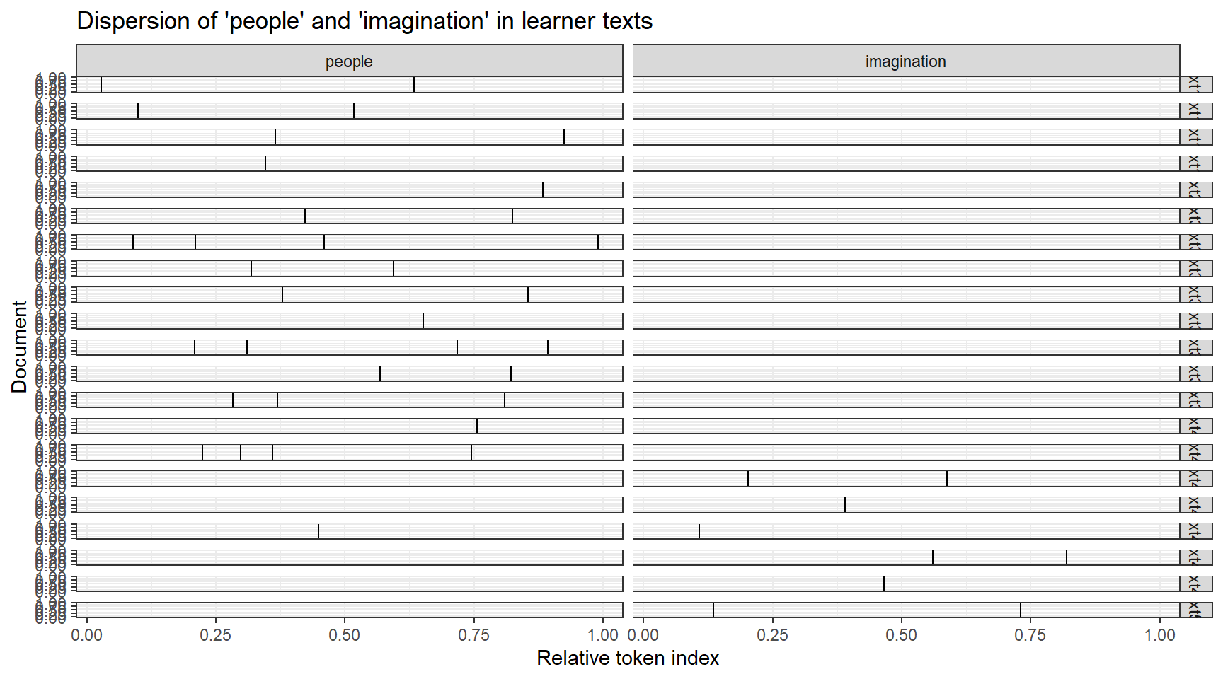
The textplot_xray() function from quanteda.textplots produces a dispersion plot (sometimes called a lexical dispersion plot) — a visual representation of where in each document a given term appears. Each vertical tick mark represents one occurrence; the horizontal axis represents the position within the document as a proportion of its total length.

# Extract KWIC for two terms to compare their dispersion across learner texts
kwic_disp <- quanteda::kwic(
  quanteda::tokens(learner),
  pattern = c("people", "imagination")
)
quanteda.textplots::textplot_xray(kwic_disp) +
  theme_bw() +
  labs(title = "Dispersion of 'people' and 'imagination' in learner texts")

Concordancing Phrases

To search for a multi-word sequence, wrap the pattern in quanteda::phrase(). The example below retrieves all instances of very followed by any single word:

kwic_very <- quanteda::kwic(
  quanteda::tokens(learner),
  pattern   = phrase("^very [a-z]{1,}"),  # "very" + any lowercase word
  valuetype = "regex"
) |>
  as.data.frame() |>
  dplyr::select(-from, -to, -pattern)

docname	pre	keyword	post
text3	in black trousers and only	very seldom	in skirts , because she
text4	is admirable is that she's	very active	in doing sports and that
text4	managed by her in a	very simple	way . She's very interested
text4	very simple way . She's	very interested	in cycling , swimming and
text5	She's also	very intelligent	and because of that she
text6	Last of all she's	very friendly	and there's nearly nobody in

When to Use Regex vs. Glob Patterns

quanteda::kwic() supports three valuetype options: "fixed" (exact string match), "glob" (wildcard with * and ?), and "regex" (full regular expression). For most single-word searches, "glob" with a trailing * (e.g. "problem*") is the simplest option. Use "regex" when you need character classes, alternation (|), or more complex patterns. Use phrase() together with "regex" for multi-word patterns.

---

Check Your Understanding: Concordancing

Q1. You want to find all instances of the phrase in my opinion in a learner corpus. Which quanteda::kwic() call is correct?

quanteda::kwic(tokens(corpus), pattern = 'in_my_opinion', valuetype = 'glob')
quanteda::kwic(tokens(corpus), pattern = 'in my opinion', valuetype = 'fixed')
quanteda::kwic(tokens(corpus), pattern = c('in', 'my', 'opinion'), valuetype = 'fixed')
quanteda::kwic(tokens(corpus), pattern = phrase('in my opinion'), valuetype = 'fixed')

---

Q2. What is the purpose of reversing the left context (stringi::stri_reverse(pre)) before sorting a concordance?

It reverses the order of concordance lines so the rarest instances appear first
It removes stopwords from the left context before sorting
It allows sorting by the word immediately to the left of the keyword, grouping instances that share the same preceding collocate
It converts the left context to uppercase for case-insensitive sorting

---

Frequency Lists

Section Overview

What you’ll learn: How to build a word frequency list from corpus text, how to remove stopwords to reveal content-word distributions, and how to visualise frequency rankings as bar charts and word clouds

Frequency lists — ranked lists of all word types and their occurrence counts — are among the most basic but informative tools in corpus linguistics. They give an immediate picture of the vocabulary profile of a text or corpus: which words are most common, how quickly frequency drops off across the vocabulary, and how a corpus’s most frequent words compare to those of another corpus. Comparing the frequency profiles of learner and native-speaker texts can reveal systematic over- or under-use of specific words or word types.

Building a Frequency List

We build a frequency list for the pooled L1 (LOCNESS) data. The pipeline removes punctuation, normalises case, splits into word tokens, and counts.

ftb <- c(ns1, ns2) |>
  stringr::str_replace_all("\\W", " ") |>   # replace non-word characters with spaces
  stringr::str_squish() |>                   # collapse multiple spaces
  tolower() |>                               # normalise to lowercase
  stringr::str_split(" ") |>                # split into word tokens
  unlist() |>
  as.data.frame() |>
  dplyr::rename(word = 1) |>
  dplyr::filter(word != "") |>
  dplyr::count(word, name = "freq") |>
  dplyr::arrange(desc(freq))

head(ftb, 10)

   word freq
1   the  650
2    to  373
3    of  320
4   and  283
5    is  186
6     a  176
7    in  162
8    be  121
9  this  120
10  are  111

The most frequent words are, unsurprisingly, grammatical function words: the, a, of, and, to. These are important for syntactic processing but carry little lexical content and are rarely of interest when studying vocabulary use.

Removing Stopwords

We use dplyr::anti_join() with the stop_words lexicon from the tidytext package to remove high-frequency function words, leaving only content words.

ftb_content <- ftb |>
  dplyr::anti_join(stop_words, by = "word")

head(ftb_content, 10)

        word freq
1  transport   98
2     people   85
3      roads   80
4       cars   69
5       road   51
6     system   50
7       rail   48
8    traffic   45
9     public   41
10    trains   36

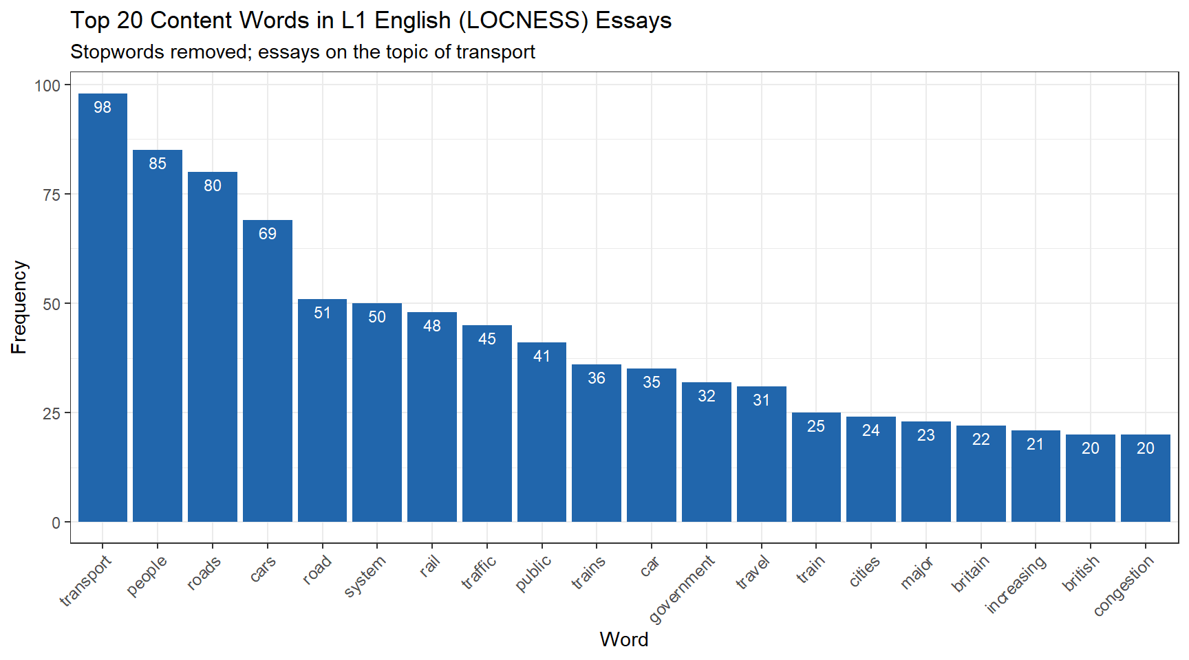
The content-word list now surfaces topically informative vocabulary. Because the essays are about transport, we expect words like transport, road, car, public, and people to feature prominently — and indeed they do. This topical coherence also serves as a useful sanity check that the data have been loaded and processed correctly.

Visualising Frequency as a Bar Chart

ftb_content |>
  head(20) |>
  ggplot(aes(x = reorder(word, -freq), y = freq, label = freq)) +
  geom_col(fill = "#2166AC") +
  geom_text(vjust = 1.5, colour = "white", size = 3) +
  theme_bw() +
  theme(axis.text.x = element_text(size = 9, angle = 45, hjust = 1)) +
  labs(
    title    = "Top 20 Content Words in L1 English (LOCNESS) Essays",
    subtitle = "Stopwords removed; essays on the topic of transport",
    x        = "Word",
    y        = "Frequency"
  )

Visualising Frequency as a Word Cloud

Word clouds provide a visually engaging alternative for communicating frequency information. Word size is proportional to frequency. They are best suited for communication and initial exploration rather than precise quantitative comparison.

wordcloud2::wordcloud2(
  ftb_content[1:100, ],
  shape = "diamond",
  color = scales::viridis_pal()(8)
)

Word Clouds Are Approximate

Word clouds encode frequency information through font size, which is difficult to compare precisely across words. They are useful for getting a quick visual impression of vocabulary but should not be used for quantitative claims. For rigorous frequency comparisons, use bar charts or tables with exact counts.

---

Check Your Understanding: Frequency Lists

Q3. You compare the raw frequency list and the content-word list for an English corpus and notice that the appears 4,200 times in the raw list but is absent from the content-word list. What caused the removal?

filter(word != '') removed it because single-character words are excluded
tolower() converted 'the' to an empty string
anti_join(stop_words) removed it because 'the' appears in the tidytext stop_words lexicon
str_replace_all('\\W', ' ') replaced 'the' with a space because it contains no vowels

---

Sentence Length

Section Overview

What you’ll learn: How to split texts into individual sentences, how to count words per sentence, and how to compare sentence length distributions across L1 groups using box plots

Key functions: tokenizers::tokenize_sentences(), tokenizers::count_words()

Average sentence length (ASL) is one of the most widely used surface measures of syntactic complexity in learner language research. Longer sentences generally involve more syntactic subordination and coordination, which are markers of greater grammatical proficiency (Kyle and Crossley 2018). Comparing ASL across L1 groups and between learners and native speakers can reveal whether certain L1 backgrounds are associated with shorter, simpler sentences or longer, more complex ones.

Splitting Texts into Sentences

We write a reusable cleaning function that removes ICLE/LOCNESS file headers, strips internal quotation marks that can confuse sentence boundary detection, and then splits the text into individual sentences using tokenizers::tokenize_sentences().

cleanText <- function(x) {
  x <- paste0(x)
  x <- stringr::str_remove_all(x, "<.*?>")         # remove XML/HTML-style tags
  x <- stringr::str_remove_all(x, fixed("\""))      # remove double quotation marks
  x <- x[x != ""]                                   # drop empty strings
  x <- tokenizers::tokenize_sentences(x)
  x <- unlist(x)
  return(x)
}

# Apply to all texts
ns1_sen <- cleanText(ns1);  ns2_sen <- cleanText(ns2)
de_sen  <- cleanText(de);   es_sen  <- cleanText(es)
fr_sen  <- cleanText(fr);   it_sen  <- cleanText(it)
pl_sen  <- cleanText(pl);   ru_sen  <- cleanText(ru)

ru_sen
It is now a very wide spread opinion, that in the modern world there is no place for dreaming and imagination.
Those who share this point of view usually say that at present we are so very much under the domination of science, industry, technology, ever-increasing tempo of our lives and so on, that neither dreaming nor imagination can possibly survive.
Their usual argument is very simple - they suggest to their opponents to look at some samples of the modern art and to compare them to the masterpieces of the Old Masters of painting, music, literature.
As everything which is simple, the argument sounds very convincing.
Of course, it is evident, that no modern writer, painter or musician can be compare to such names as Bach, Pushkin< Byron, Mozart, Rembrandt, Raffael et cetera.

Computing Sentence Lengths

tokenizers::count_words() returns the number of whitespace-delimited tokens in each sentence. We collect these counts into a single data frame with an l1 column identifying the speaker group.

sl_df <- data.frame(
  sentenceLength = c(
    tokenizers::count_words(ns1_sen), tokenizers::count_words(ns2_sen),
    tokenizers::count_words(de_sen),  tokenizers::count_words(es_sen),
    tokenizers::count_words(fr_sen),  tokenizers::count_words(it_sen),
    tokenizers::count_words(pl_sen),  tokenizers::count_words(ru_sen)
  ),
  l1 = c(
    rep("en", tokenizers::count_words(ns1_sen) |> length()),
    rep("en", tokenizers::count_words(ns2_sen) |> length()),
    rep("de", tokenizers::count_words(de_sen) |> length()),
    rep("es", tokenizers::count_words(es_sen) |> length()),
    rep("fr", tokenizers::count_words(fr_sen) |> length()),
    rep("it", tokenizers::count_words(it_sen) |> length()),
    rep("pl", tokenizers::count_words(pl_sen) |> length()),
    rep("ru", tokenizers::count_words(ru_sen) |> length())
  )
)

head(sl_df)

  sentenceLength l1
1              2 en
2             17 en
3             23 en
4             17 en
5             20 en
6             34 en

Visualising Sentence Length Distributions

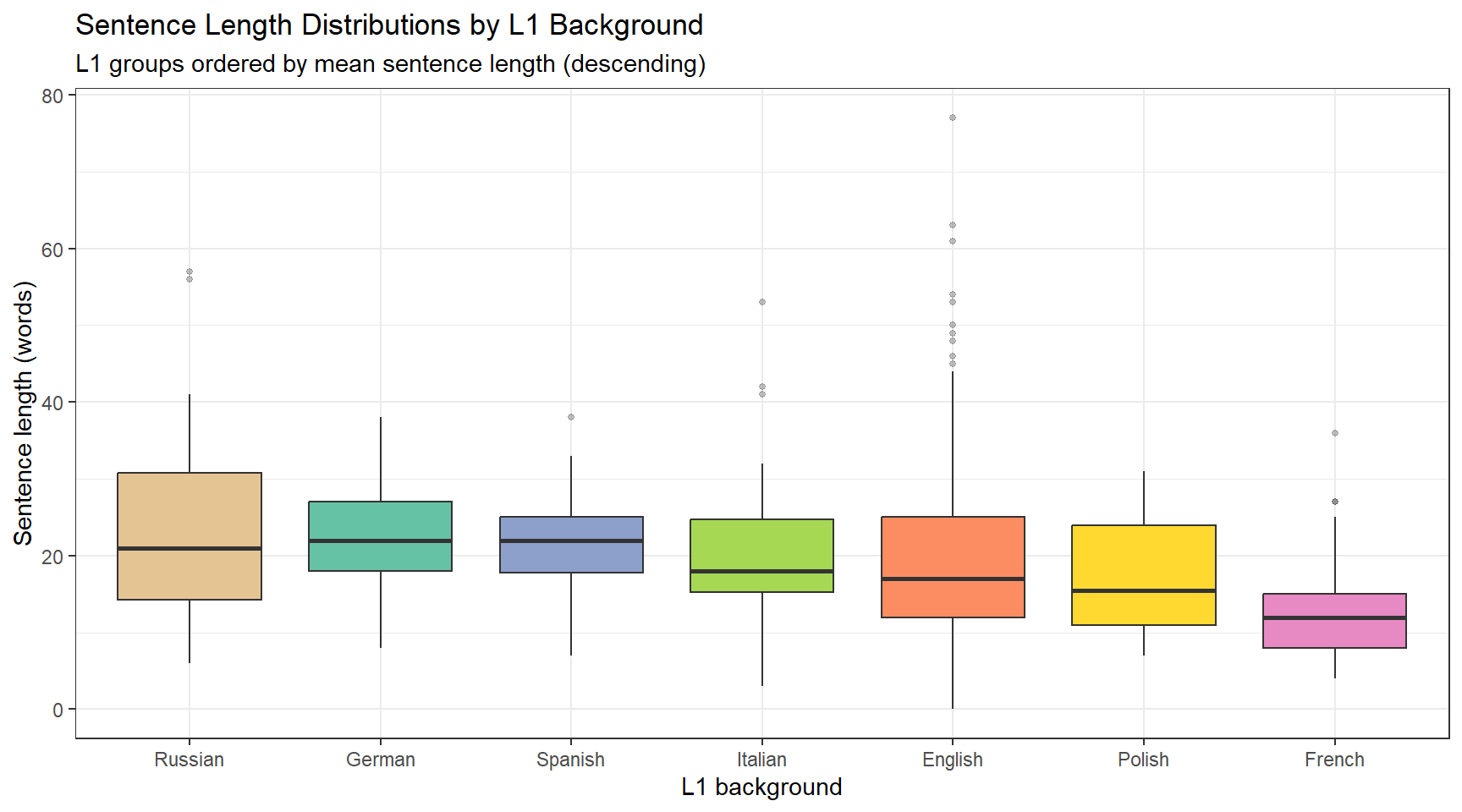
Box plots are ideal for comparing distributions across groups: they display the median, interquartile range, and outliers simultaneously, making differences in central tendency and spread immediately visible.

l1_labels <- c("en" = "English", "de" = "German", "es" = "Spanish",
                "fr" = "French",  "it" = "Italian", "pl" = "Polish", "ru" = "Russian")

sl_df |>
  ggplot(aes(x = reorder(l1, -sentenceLength, mean), y = sentenceLength, fill = l1)) +
  geom_boxplot(outlier.alpha = 0.3, outlier.size = 1) +
  scale_x_discrete("L1 background", labels = l1_labels) +
  scale_fill_brewer(palette = "Set2", guide = "none") +
  theme_bw() +
  labs(
    title    = "Sentence Length Distributions by L1 Background",
    subtitle = "L1 groups ordered by mean sentence length (descending)",
    y        = "Sentence length (words)"
  )

The plot reveals considerable variation both within and across groups. L1 English speakers tend to produce longer sentences on average than most learner groups, which may reflect greater syntactic command of subordination and embedding. However, the wide interquartile ranges and overlapping distributions remind us that sentence length alone is a noisy and indirect indicator of proficiency — a very short sentence may be stylistically deliberate, and a very long sentence may be run-on or poorly constructed.

---

Check Your Understanding: Sentence Length

Q4. A researcher finds that Polish learners produce significantly shorter sentences than L1 English speakers on average. Which of the following would be the most appropriate immediate follow-up analysis?

Replace sentence length with word length as the complexity measure, since word length is more reliable
Conclude that Polish learners have lower English proficiency than other groups, since sentence length is a direct measure of proficiency
Remove all sentences shorter than 5 words from the Polish data to eliminate noise before re-running the analysis
Examine the syntactic structure of Polish learner sentences (e.g., rates of subordinate clauses) to determine whether shorter sentences reflect less syntactic complexity or a different discourse style

---

N-gram Analysis

Section Overview

What you’ll learn: How to extract word bigrams from corpus texts, how to normalise their frequencies for cross-corpus comparison, and how to identify which bigrams are used significantly more or less often by learners compared to L1 speakers using Fisher’s exact test with Bonferroni correction

Key functions: quanteda::tokens_ngrams(), fisher.test()

N-grams are contiguous sequences of n words. Bigrams (2-grams) capture word pairs; trigrams (3-grams) capture three-word sequences; and so on. N-gram analysis is used in learner corpus research to identify formulaic sequences — multi-word units that learners may use differently from native speakers. Over-use or under-use of certain bigrams can indicate L1 transfer effects, limited access to target-language formulaic sequences, or avoidance of specific collocational patterns.

Extracting Bigrams

We tokenise each sentence set, apply tokens_ngrams(n = 2), and then build a unified data frame with an l1 column and a binary learner column.

# Tokenise (lowercase, punctuation removed)
tok_list <- list(
  ns1 = quanteda::tokens(tolower(ns1_sen), remove_punct = TRUE),
  ns2 = quanteda::tokens(tolower(ns2_sen), remove_punct = TRUE),
  de  = quanteda::tokens(tolower(de_sen),  remove_punct = TRUE),
  es  = quanteda::tokens(tolower(es_sen),  remove_punct = TRUE),
  fr  = quanteda::tokens(tolower(fr_sen),  remove_punct = TRUE),
  it  = quanteda::tokens(tolower(it_sen),  remove_punct = TRUE),
  pl  = quanteda::tokens(tolower(pl_sen),  remove_punct = TRUE),
  ru  = quanteda::tokens(tolower(ru_sen),  remove_punct = TRUE)
)

# Extract bigrams for each group
bigram_list <- lapply(tok_list, function(x)
  as.vector(unlist(quanteda::tokens_ngrams(x, n = 2)))
)

# Inspect a sample
head(bigram_list$ns1, 10)

 [1] "transport_01"   "the_basic"      "basic_dilema"   "dilema_facing" 
 [5] "facing_the"     "the_uk's"       "uk's_rail"      "rail_and"      
 [9] "and_road"       "road_transport"

# Build unified data frame
ngram_df <- data.frame(
  ngram   = unlist(bigram_list),
  l1      = rep(names(bigram_list), sapply(bigram_list, length)),
  learner = ifelse(rep(names(bigram_list), sapply(bigram_list, length)) == "ns1" |
                   rep(names(bigram_list), sapply(bigram_list, length)) == "ns2",
                   "no", "yes")
)

head(ngram_df)

             ngram  l1 learner
ns11  transport_01 ns1      no
ns12     the_basic ns1      no
ns13  basic_dilema ns1      no
ns14 dilema_facing ns1      no
ns15    facing_the ns1      no
ns16      the_uk's ns1      no

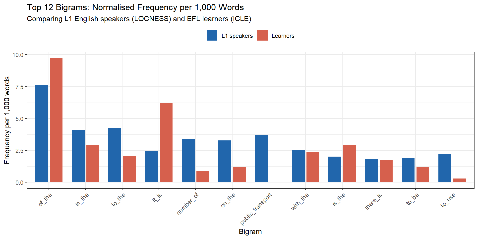
Normalising Frequencies

Because the L1 and learner sub-corpora differ in total word count, we cannot compare raw bigram frequencies directly. We normalise to per-1,000-word rates by dividing each group’s bigram count by the total number of bigrams produced by that group, then multiplying by 1,000.

# Count bigrams per learner/L1 group
ngram_freq <- ngram_df |>
  dplyr::group_by(ngram, learner) |>
  dplyr::summarise(freq = dplyr::n(), .groups = "drop") |>
  dplyr::arrange(desc(freq))

# Add normalised frequencies
ngram_norm <- ngram_freq |>
  dplyr::group_by(ngram) |>
  dplyr::mutate(total_ngram = sum(freq)) |>
  dplyr::group_by(learner) |>
  dplyr::mutate(
    total_group = sum(freq),
    rfreq       = freq / total_group * 1000
  ) |>
  dplyr::ungroup()

# Spread to wide format (one column per group), fill missing with 0
ngram_wide <- ngram_norm |>
  dplyr::select(ngram, learner, rfreq, total_ngram) |>
  tidyr::pivot_wider(names_from = learner, values_from = rfreq,
                     values_fill = 0) |>
  dplyr::arrange(desc(total_ngram))

head(ngram_wide, 10)

# A tibble: 10 × 4
   ngram            total_ngram    no   yes
   <chr>                  <int> <dbl> <dbl>
 1 of_the                   105  7.62 9.72 
 2 in_the                    49  4.13 2.95 
 3 to_the                    47  4.23 2.06 
 4 it_is                     44  2.43 6.19 
 5 public_transport          35  3.70 0    
 6 number_of                 35  3.39 0.884
 7 on_the                    35  3.28 1.18 
 8 with_the                  32  2.54 2.36 
 9 is_the                    29  2.01 2.95 
10 there_is                  23  1.80 1.77 

Visualising the Most Frequent Bigrams

ngram_norm |>
  dplyr::select(ngram, learner, rfreq, total_ngram) |>
  tidyr::pivot_wider(names_from = learner, values_from = rfreq, values_fill = 0) |>
  dplyr::arrange(desc(total_ngram)) |>
  head(12) |>
  tidyr::pivot_longer(cols = c(no, yes), names_to = "learner", values_to = "rfreq") |>
  dplyr::mutate(learner = dplyr::recode(learner, "no" = "L1 speakers", "yes" = "Learners")) |>
  ggplot(aes(x = reorder(ngram, -total_ngram), y = rfreq, fill = learner)) +
  geom_col(position = position_dodge(width = 0.8), width = 0.7) +
  scale_fill_manual(values = c("L1 speakers" = "#2166AC", "Learners" = "#D6604D")) +
  theme_bw() +
  theme(axis.text.x = element_text(angle = 45, hjust = 1, size = 9),
        legend.position = "top") +
  labs(
    title    = "Top 12 Bigrams: Normalised Frequency per 1,000 Words",
    subtitle = "Comparing L1 English speakers (LOCNESS) and EFL learners (ICLE)",
    x        = "Bigram",
    y        = "Frequency per 1,000 words",
    fill     = NULL
  )

Testing for Significant Differences

Visual comparison is informative but we need a statistical test to determine which differences are unlikely to be due to chance. We use Fisher’s exact test, which is appropriate for count data in 2×2 contingency tables. For each bigram, the table compares: (a) its count in L1 data vs. (b) all other bigrams in L1 data, against (c) its count in learner data vs. (d) all other bigrams in learner data.

Because we run one test per bigram (potentially thousands of tests), we apply a Bonferroni correction: the critical p-value is divided by the number of tests, making the threshold much more stringent and controlling the family-wise error rate.

# Reshape for Fisher's test: one row per bigram, counts for each group
fisher_df <- ngram_freq |>
  tidyr::pivot_wider(names_from = learner, values_from = freq, values_fill = 0) |>
  dplyr::rename(l1speaker = no, learner = yes) |>
  dplyr::ungroup() |>
  dplyr::mutate(
    total_l1      = sum(l1speaker),
    total_learner = sum(learner),
    a = l1speaker,
    b = learner,
    c = total_l1      - l1speaker,
    d = total_learner - learner
  )

# Apply Fisher's exact test row-wise; add Bonferroni correction
fisher_results <- fisher_df |>
  dplyr::rowwise() |>
  dplyr::mutate(
    fisher_p   = fisher.test(matrix(c(a, c, b, d), nrow = 2))$p.value,
    odds_ratio = fisher.test(matrix(c(a, c, b, d), nrow = 2))$estimate,
    crit       = 0.05 / nrow(fisher_df),
    sig_corr   = ifelse(fisher_p < crit, "p < .05*", "n.s.")
  ) |>
  dplyr::ungroup() |>
  dplyr::arrange(fisher_p) |>
  dplyr::select(ngram, l1speaker, learner, fisher_p, odds_ratio, sig_corr)

head(fisher_results, 10)

# A tibble: 10 × 6
   ngram            l1speaker learner  fisher_p odds_ratio sig_corr
   <chr>                <int>   <int>     <dbl>      <dbl> <chr>   
 1 in_silence               0       8 0.0000236          0 n.s.    
 2 public_transport        35       0 0.0000276        Inf n.s.    
 3 silence_is               0       7 0.0000896          0 n.s.    
 4 of_all                   0       6 0.000339           0 n.s.    
 5 our_society              0       6 0.000339           0 n.s.    
 6 in_our                   0       5 0.00129            0 n.s.    
 7 in_prison                0       5 0.00129            0 n.s.    
 8 of_guns                  0       5 0.00129            0 n.s.    
 9 people_can               0       5 0.00129            0 n.s.    
10 the_gulf                 0       5 0.00129            0 n.s.    

# How many bigrams reach significance after Bonferroni correction?
table(fisher_results$sig_corr)

n.s. 
9036 

Interpreting Fisher’s Exact Test Results

A significant result (p < Bonferroni-corrected threshold) means that the observed difference in bigram frequency between learners and L1 speakers is unlikely to have arisen by chance, given the corpus sizes. The odds ratio indicates the direction: an odds ratio > 1 means the bigram is proportionally more common in L1 speech; an odds ratio < 1 means it is proportionally more common in learner speech.

In small sub-corpora like the present data, it is common to find few or no significant results after Bonferroni correction, because the test is very conservative when the number of comparisons is large. Larger corpora or a less conservative correction (e.g. the Benjamini-Hochberg false discovery rate procedure) would typically reveal more significant differences.

---

Check Your Understanding: N-gram Analysis

Q5. Why is Bonferroni correction necessary when testing bigram frequency differences across an entire frequency list?

It is required to convert Fisher's exact test p-values into odds ratios
Without correction, the odds ratios would be biased toward values greater than 1
Bonferroni correction increases statistical power by pooling information across all tests
Running many tests simultaneously inflates the probability of finding at least one false positive by chance; Bonferroni correction adjusts the critical p-value downward to control the family-wise error rate

---

Collocations and Collocation Networks

Section Overview

What you’ll learn: How to identify statistically significant word collocations using log-likelihood, how to build a feature co-occurrence matrix, and how to visualise collocational relationships as a network graph

Key functions: quanteda.textstats::textstat_collocations(), quanteda::fcm(), quanteda.textplots::textplot_network()

A collocation is a pair (or larger group) of words that co-occur more frequently than chance would predict. Identifying collocations is important in learner language research because learners often struggle with the conventional collocational patterns of the target language — they may produce grammatically correct but collocationally unusual combinations (e.g. make homework instead of do homework) that mark their output as non-native (Nesselhauf 2005).

Identifying Collocations

We use quanteda.textstats::textstat_collocations(), which computes the lambda statistic (a log-likelihood-based association measure) for all word pairs appearing at least min_count times. Higher lambda values indicate stronger association — the pair co-occurs much more frequently than expected by chance.

# Combine L1 sentences and tokenise
ns_sen   <- c(ns1_sen, ns2_sen)
ns_tokens <- quanteda::tokens(tolower(ns_sen), remove_punct = TRUE)

# Identify collocations occurring at least 20 times
ns_coll <- quanteda.textstats::textstat_collocations(ns_tokens, size = 2, min_count = 20)

collocation	count	count_nested	length	lambda	z
public transport	35	0	2	7.1702271	14.899245
it is	23	0	2	3.1190429	12.152647
of the	72	0	2	1.6178618	11.456242
to use	21	0	2	3.4556530	10.583556
number of	32	0	2	5.6938299	10.063860
on the	31	0	2	2.1031266	9.433550
in the	39	0	2	1.6728346	8.874487
with the	24	0	2	2.3004624	8.817610
the number	20	0	2	2.9141572	8.593513
to the	40	0	2	0.6685972	3.880229

The strongest collocations in this transport-themed corpus include named entities and set phrases specific to the topic. This is typical for domain-specific corpora: the most frequent collocations tend to be topically coherent multi-word units.

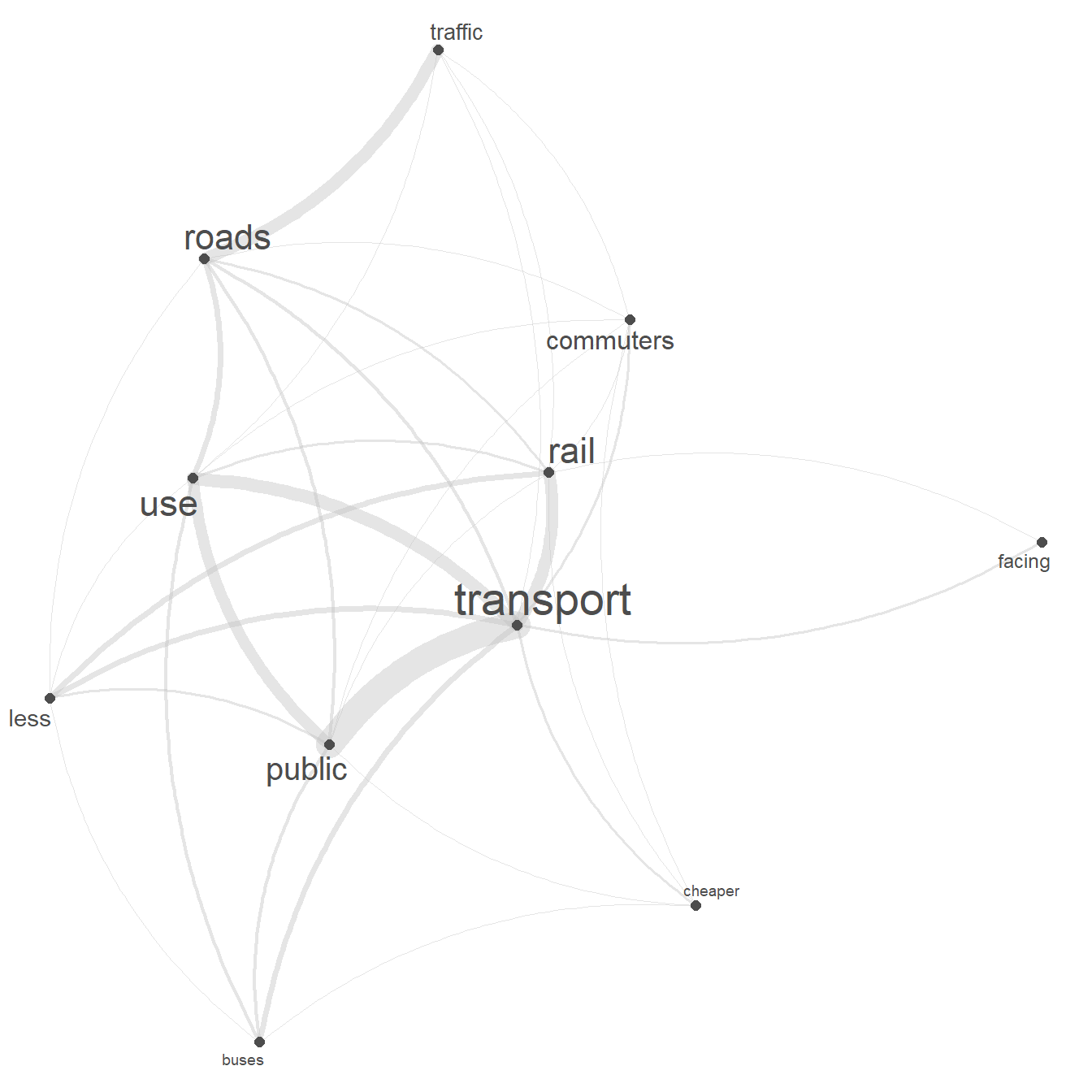
Building a Collocation Network

A collocation network visualises the collocational relationships around a target term as a graph, where nodes are words and edges represent co-occurrence strength. This makes it easy to see at a glance which words cluster together around a focal term.

External Script Dependency

The code below uses the calculateCoocStatistics() function, which is not part of any CRAN package. It is available as a standalone R script (rscripts/calculateCoocStatistics.R) in the LADAL repository. Download it from the LADAL GitHub repository and place it in a sub-folder called rscripts/ within your R project before running this section. The function calculates log-likelihood-based co-occurrence statistics between a target term and all other terms in a Document-Feature Matrix.

# Build a DFM from the L1 sentences (stopwords removed)
ns_dfm <- quanteda::dfm(
  quanteda::tokens(ns_sen, remove_punct = TRUE)
) |>
  quanteda::dfm_remove(pattern = stopwords("english"))

# Load the co-occurrence statistics function
source("rscripts/calculateCoocStatistics.R")

# Compute log-likelihood co-occurrence statistics for the target term "transport"
coocTerm <- "transport"
coocs    <- calculateCoocStatistics(coocTerm, ns_dfm, measure = "LOGLIK")

# Inspect the top 10 collocates
coocs[1:10]

    public        use    traffic       rail     facing  commuters    cheaper 
113.171974  19.437311  10.508626   9.652830   9.382889   9.382889   9.382889 
     roads       less      buses 
  9.080648   8.067363   6.702863 

# Reduce DFM to the top 10 collocates plus the target word
redux_dfm <- quanteda::dfm_select(
  ns_dfm,
  pattern = c(names(coocs)[1:10], coocTerm)
)

# Convert to Feature Co-occurrence Matrix (FCM)
# FCM[i,j] = number of documents in which word i and word j both appear
tag_fcm <- quanteda::fcm(redux_dfm)

# Visualise the collocation network
quanteda.textplots::textplot_network(
  tag_fcm,
  min_freq        = 1,
  edge_alpha      = 0.4,
  edge_size       = 5,
  edge_color      = "gray75",
  vertex_labelsize = log(rowSums(tag_fcm) * 12)
)

In the network, the size of each node’s label is proportional to its overall frequency in the DFM (a log-scaled version of the row sums). Edges between nodes represent co-occurrence in the same document. The target term transport should appear as the most central node, with the strongest edges connecting to its most frequent and most strongly associated collocates.

---

Check Your Understanding: Collocations

Q6. A learner writes “she did a big mistake” instead of the native-speaker form “she made a big mistake”. What type of error does this represent, and which corpus analysis method would be most appropriate to study it systematically?

A lexical diversity error; TTR analysis would reveal that the learner is using a less varied vocabulary
A spelling error; hunspell spell-checking would detect and count these systematically
A sentence length error; the sentence is too short relative to the L1 norm
A collocational error (wrong verb choice in a verb-noun collocation); collocation analysis comparing learner and L1 frequencies of verb-noun pairs would identify systematic differences in verb selection

---

Part-of-Speech Tagging and POS-Sequence Analysis

Section Overview

What you’ll learn: How to automatically assign part-of-speech tags to corpus texts using udpipe, how to extract POS-tag bigrams, how to compare their frequencies between learners and L1 speakers, and how to use KWIC to inspect the actual words behind significant differences

Key package: udpipe

Part-of-speech (POS) tagging is the automatic assignment of grammatical category labels (noun, verb, adjective, etc.) to each token in a text. Comparing POS-tag sequences between learner and native-speaker texts reveals grammatical differences that are invisible at the word level — for example, differences in the rate of adjective use, the frequency of passive constructions, or the distribution of subordinating conjunctions. POS-based analysis is particularly powerful for studying grammatical complexity and for identifying constructions that transfer from the learner’s L1.

Required: udpipe Language Model

This section requires a pre-trained udpipe language model for English. If you have not already downloaded it, run the following code once:

m_eng <- udpipe::udpipe_download_model(language = "english-ewt")

This downloads the English EWT (English Web Treebank) model to your working directory. Subsequent sessions should load it directly using udpipe_load_model() with the path to the downloaded .udpipe file, as shown below. The file is approximately 16 MB. Do not re-download it in every session — the download creates a local copy that persists between sessions.

Testing POS Tagging on a Sample Sentence

Before tagging the full corpus, we test the tagger on a single sentence to inspect the output format and verify that tagging is working as expected.

# Load the pre-downloaded English EWT model
m_eng <- udpipe::udpipe_load_model(
  file = here::here("udpipemodels", "english-ewt-ud-2.5-191206.udpipe")
)

# Tag a test sentence
test_sentence <- "It is now a very wide-spread opinion that in the modern world there is no place for dreaming and imagination."

tagged_test <- udpipe::udpipe_annotate(m_eng, x = test_sentence) |>
  as.data.frame() |>
  dplyr::select(token, upos, xpos, dep_rel)

head(tagged_test, 12)

     token  upos xpos  dep_rel
1       It  PRON  PRP    nsubj
2       is   AUX  VBZ      cop
3      now   ADV   RB   advmod
4        a   DET   DT      det
5     very   ADV   RB   advmod
6     wide   ADJ   JJ     amod
7        - PUNCT HYPH    punct
8   spread  NOUN   NN compound
9  opinion  NOUN   NN     root
10    that  PRON  WDT      obj
11      in   ADP   IN     case
12     the   DET   DT      det

The output contains several annotation columns. upos is the Universal POS tag (a coarse, cross-linguistically consistent tag set: NOUN, VERB, ADJ, etc.). xpos is the Penn Treebank tag (a finer-grained English-specific tag set: NN, VBZ, JJ, etc.). dep_rel is the dependency relation label. For our bigram analysis we use xpos tags, in which adjectives are tagged JJ, present-tense verbs VBZ, personal pronouns PRP, and so on.

We create a tagged version of the text by concatenating each token with its xpos tag, separated by /:

tagged_str <- paste0(tagged_test$token, "/", tagged_test$xpos, collapse = " ")
tagged_str

[1] "It/PRP is/VBZ now/RB a/DT very/RB wide/JJ -/HYPH spread/NN opinion/NN that/WDT in/IN the/DT modern/JJ world/NN there/EX is/VBZ no/DT place/NN for/IN dreaming/VBG and/CC imagination/NN ./."

Tagging All Texts

We write a function comText() that cleans a text, runs udpipe annotation, and returns the token/tag string. We then apply it to all eight text sets.

comText <- function(x) {
  x <- paste0(x, collapse = " ")
  x <- stringr::str_remove_all(x, "<.*?>")       # remove markup tags
  x <- stringr::str_remove_all(x, fixed("\""))    # remove quotation marks
  x <- stringr::str_squish(x)
  x <- x[x != ""]
  annotated <- udpipe::udpipe_annotate(m_eng, x = x) |>
    as.data.frame()
  paste0(annotated$token, "/", annotated$xpos, collapse = " ")
}

# Apply to all texts (this step takes a few minutes per text)
ns1_pos <- comText(ns1_sen);  ns2_pos <- comText(ns2_sen)
de_pos  <- comText(de_sen);   es_pos  <- comText(es_sen)
fr_pos  <- comText(fr_sen);   it_pos  <- comText(it_sen)
pl_pos  <- comText(pl_sen);   ru_pos  <- comText(ru_sen)

# Preview the first 300 characters of the L1 tagged text
substr(ns1_pos, 1, 300)

[1] "Transport/NNP 01/CD The/DT basic/JJ dilema/NN facing/VBG the/DT UK/NNP 's/POS rail/NN and/CC road/NN transport/NN system/NN is/VBZ the/DT general/JJ rise/NN in/IN population/NN ./. This/DT leads/VBZ to/IN an/DT increase/NN in/IN the/DT number/NN of/IN commuters/NNS and/CC transport/NN users/NNS ever"

Extracting POS-Tag Bigrams

We extract bigrams of POS tags only (stripping the word tokens) and tabulate their frequencies for learners and L1 speakers.

# Function: strip word tokens, keep only POS tags, extract tag bigrams
posngram <- function(x) {
  x |>
    stringr::str_remove_all("\\w*/") |>          # remove "word/" prefix from each token
    quanteda::tokens(remove_punct = TRUE) |>
    quanteda::tokens_ngrams(n = 2)
}

# Apply and unlist
ns1_posng <- as.vector(unlist(posngram(ns1_pos)))
ns2_posng <- as.vector(unlist(posngram(ns2_pos)))
de_posng  <- as.vector(unlist(posngram(de_pos)))
es_posng  <- as.vector(unlist(posngram(es_pos)))
fr_posng  <- as.vector(unlist(posngram(fr_pos)))
it_posng  <- as.vector(unlist(posngram(it_pos)))
pl_posng  <- as.vector(unlist(posngram(pl_pos)))
ru_posng  <- as.vector(unlist(posngram(ru_pos)))

head(ns1_posng, 8)

[1] "NNP_CD"  "CD_DT"   "DT_JJ"   "JJ_NN"   "NN_VBG"  "VBG_DT"  "DT_NNP" 
[8] "NNP_POS"

# Build unified table with learner/L1 labels
posngram_df <- data.frame(
  ngram   = c(ns1_posng, ns2_posng, de_posng, es_posng,
              fr_posng,  it_posng,  pl_posng,  ru_posng),
  l1      = c(rep("en", length(ns1_posng)), rep("en", length(ns2_posng)),
              rep("de", length(de_posng)),  rep("es", length(es_posng)),
              rep("fr", length(fr_posng)),  rep("it", length(it_posng)),
              rep("pl", length(pl_posng)),  rep("ru", length(ru_posng))),
  learner = ifelse(
    c(rep("en", length(ns1_posng) + length(ns2_posng)),
      rep("l2", length(de_posng)  + length(es_posng) +
                length(fr_posng)  + length(it_posng) +
                length(pl_posng)  + length(ru_posng))) == "en",
    "no", "yes")
) |>
  dplyr::group_by(ngram, learner) |>
  dplyr::summarise(freq = dplyr::n(), .groups = "drop") |>
  dplyr::arrange(desc(freq))

head(posngram_df, 8)

# A tibble: 8 × 3
  ngram  learner  freq
  <chr>  <chr>   <int>
1 DT_NN  no        520
2 IN_DT  no        465
3 NN_IN  no        465
4 JJ_NN  no        334
5 IN_NN  no        241
6 DT_JJ  no        236
7 TO_VB  no        235
8 NNS_IN no        222

Testing for Significant POS-Sequence Differences

We apply the same Fisher’s exact test + Bonferroni correction approach as in the N-gram section, but now operating on POS-tag bigrams rather than word bigrams.

posng_fisher <- posngram_df |>
  tidyr::pivot_wider(names_from = learner, values_from = freq, values_fill = 0) |>
  dplyr::rename(l1speaker = no, learner = yes) |>
  dplyr::ungroup() |>
  dplyr::mutate(
    total_l1      = sum(l1speaker),
    total_learner = sum(learner),
    a = l1speaker,
    b = learner,
    c = total_l1      - l1speaker,
    d = total_learner - learner
  )

bonferroni_crit <- 0.05 / nrow(posng_fisher)

posng_fisher <- posng_fisher |>
  dplyr::rowwise() |>
  dplyr::mutate(
    fisher_p   = fisher.test(matrix(c(a, c, b, d), nrow = 2))$p.value,
    odds_ratio = fisher.test(matrix(c(a, c, b, d), nrow = 2))$estimate,
    sig_corr   = ifelse(fisher_p < bonferroni_crit, "p < .05*", "n.s.")
  ) |>
  dplyr::ungroup() |>
  dplyr::arrange(fisher_p) |>
  dplyr::select(ngram, l1speaker, learner, fisher_p, odds_ratio, sig_corr)

head(posng_fisher, 10)

# A tibble: 10 × 6
   ngram   l1speaker learner      fisher_p odds_ratio sig_corr
   <chr>       <int>   <int>         <dbl>      <dbl> <chr>   
 1 PRP_VBZ        43      55 0.00000000112      0.282 p < .05*
 2 $_NN           33      40 0.000000397        0.299 p < .05*
 3 NN_PRP         36      41 0.000000843        0.318 p < .05*
 4 NN_NNS        152      21 0.00000364         2.67  p < .05*
 5 IN_PRP         97      71 0.0000140          0.494 p < .05*
 6 PRP_IN          6      15 0.0000244          0.146 p < .05*
 7 JJR_NNS        42       1 0.0000391         15.4   p < .05*
 8 PRP_$          80      60 0.0000452          0.483 p < .05*
 9 NNS_VBG        37       1 0.000157          13.5   n.s.    
10 WP_VBZ          3      10 0.000231           0.109 n.s.    

Inspecting Significant POS Sequences with KWIC

When a POS-tag bigram differs significantly between groups, the next step is to inspect the actual word tokens that realise that sequence using KWIC. For example, the sequence PRP_VBZ (personal pronoun + third-person singular present verb, as in she runs, it matters) can be searched directly in the tagged text.

# Combine L1 and L2 tagged texts
l1_pos <- c(ns1_pos, ns2_pos)
l2_pos <- c(de_pos, es_pos, fr_pos, it_pos, pl_pos, ru_pos)

# KWIC for PRP_VBZ in L1 data
PRP_VBZ_l1 <- quanteda::kwic(
  quanteda::tokens(l1_pos),
  pattern   = phrase("\\w*/PRP \\w*/VBZ"),
  valuetype = "regex",
  window    = 8
) |>
  as.data.frame() |>
  dplyr::select(-from, -to, -docname, -pattern)

head(PRP_VBZ_l1, 6)

[1] pre     keyword post   
<0 rows> (or 0-length row.names)

# KWIC for PRP_VBZ in learner data
PRP_VBZ_l2 <- quanteda::kwic(
  quanteda::tokens(l2_pos),
  pattern   = phrase("\\w*/PRP \\w*/VBZ"),
  valuetype = "regex",
  window    = 8
) |>
  as.data.frame() |>
  dplyr::select(-from, -to, -docname, -pattern)

head(PRP_VBZ_l2, 6)

[1] pre     keyword post   
<0 rows> (or 0-length row.names)

Comparing the two concordances reveals whether the same syntactic pattern is associated with different lexical choices in learner and L1 production — for instance, whether learners favour different pronoun–verb combinations or use the pattern in different pragmatic contexts.

---

Check Your Understanding: POS Tagging

Q7. Why do we strip the word tokens (e.g. convert it/PRP to just PRP) before extracting POS-tag bigrams in the sequence analysis?

Because the POS tags are on the left side of the / separator and the function only reads the left side
Because including word tokens would make the bigrams too long to store efficiently in memory
Because we want to compare abstract grammatical patterns (sequences of word classes) rather than specific word combinations — removing the tokens makes every instance of the same POS sequence comparable regardless of which words realise it
Because udpipe tags contain encoding errors that cause problems if the word form is retained

---

Lexical Diversity and Readability

Section Overview

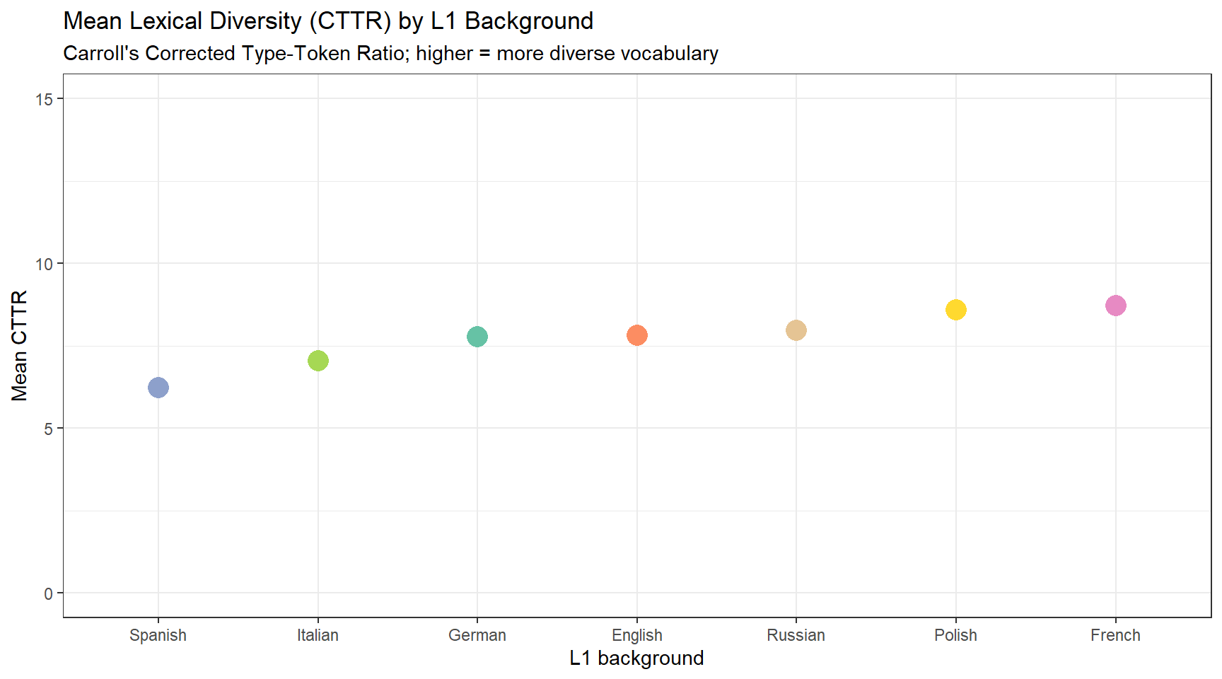
What you’ll learn: How to compute multiple lexical diversity measures (TTR, CTTR, Herdan’s C, Guiraud’s R, Maas) and Flesch readability scores for each essay, and how to compare these measures across L1 groups

Key packages: koRpus, quanteda.textstats

Lexical Diversity

Lexical diversity refers to the range and variety of vocabulary used in a text. It is considered an important indicator of L2 proficiency: more proficient learners tend to deploy a wider range of word types and rely less heavily on a small set of high-frequency forms (Daller et al. 2007). Numerous measures of lexical diversity have been proposed, each capturing a slightly different aspect of vocabulary range:

Lexical diversity measures

Measure	Formula	Notes
TTR	V / N	Types / Tokens; decreases with text length
CTTR	V / √(2N)	Carroll’s Corrected TTR; partially controls for length
C (Herdan)	log(V) / log(N)	LogTTR; more robust to length than TTR
R (Guiraud)	V / √N	Root TTR
U (Dugast)	log²(N) / (log(N) − log(V))	Uber index
Maas	(log(N) − log(V)) / log²(N)	Inverse measure; lower = more diverse

Splitting Texts into Individual Essays

Before computing lexical diversity, we split each text file into individual essays. In the ICLE/LOCNESS data, essays are separated by headers of the form Transport 01, Transport 02, etc.

cleanEss <- function(x) {
  x |>
    paste0(collapse = " ") |>
    stringr::str_split("Transport [0-9]{1,2}") |>
    unlist() |>
    stringr::str_squish() |>
    (\(v) v[v != ""])()
}

ns1_ess <- cleanEss(ns1);  ns2_ess <- cleanEss(ns2)
de_ess  <- cleanEss(de);   es_ess  <- cleanEss(es)
fr_ess  <- cleanEss(fr);   it_ess  <- cleanEss(it)
pl_ess  <- cleanEss(pl);   ru_ess  <- cleanEss(ru)

# Preview the first essay from the L1 data
substr(ns1_ess[1], 1, 400)

[1] "The basic dilema facing the UK's rail and road transport system is the general rise in population. This leads to an increase in the number of commuters and transport users every year, consequently putting pressure on the UKs transports network. The biggest worry to the system is the rapid rise of car users outside the major cities. Most large cities have managed to incourage commuters to use publi"

Computing Lexical Diversity Measures

We use koRpus::lex.div(), which computes multiple lexical diversity measures simultaneously. The segment and window arguments control the size of the moving window used for measures that are computed incrementally.

# Build a DFM from individual essays, one document per essay
all_ess <- c(ns1_ess, ns2_ess, de_ess, es_ess, fr_ess, it_ess, pl_ess, ru_ess)

ess_dfm <- quanteda::dfm(
  quanteda::tokens(all_ess, remove_punct = TRUE)
)

# Compute lexical diversity measures
ld_all <- quanteda.textstats::textstat_lexdiv(
  ess_dfm,
  measure = c("TTR", "C", "R", "CTTR", "U", "Maas")
)

# Add L1 labels
ld_all$l1 <- c(
  rep("en", length(ns1_ess) + length(ns2_ess)),
  rep("de", length(de_ess)),
  rep("es", length(es_ess)),
  rep("fr", length(fr_ess)),
  rep("it", length(it_ess)),
  rep("pl", length(pl_ess)),
  rep("ru", length(ru_ess))
)

head(ld_all)

  document       TTR         C         R     CTTR        U      Maas     lgV0
1    text1 0.6157407 0.9097853  9.049504 6.398965 25.87664 0.1965831 5.116738
2    text2 0.4751067 0.8864721 12.597049 8.907458 25.07714 0.1996921 5.453424
3    text3 0.4556765 0.8784481 11.554792 8.170472 23.10298 0.2080492 5.162563
4    text4 0.4669967 0.8811538 11.496089 8.128963 23.41239 0.2066699 5.185348
5    text5 0.4400716 0.8702500 10.404691 7.357228 21.17466 0.2173161 4.853603
6    text6 0.5197133 0.8965147 12.276679 8.680923 26.54130 0.1941060 5.558286
     lgeV0 l1
1 11.78172 en
2 12.55697 en
3 11.88724 en
4 11.93970 en
5 11.17583 en
6 12.79843 en

Extracting and Visualising CTTR

We focus on Carroll’s Corrected TTR (CTTR) as a representative lexical diversity measure. Higher CTTR values indicate greater lexical diversity.

# Extract CTTR values from the textstat_lexdiv output; add L1 labels
cttr <- ld_all |>
  dplyr::select(l1, CTTR)

head(cttr)

  l1     CTTR
1 en 6.398965
2 en 8.907458
3 en 8.170472
4 en 8.128963
5 en 7.357228
6 en 8.680923

cttr |>
  dplyr::group_by(l1) |>
  dplyr::summarise(CTTR = mean(CTTR, na.rm = TRUE), .groups = "drop") |>
  ggplot(aes(x = reorder(l1, CTTR), y = CTTR, colour = l1)) +
  geom_point(size = 5) +
  scale_x_discrete(labels = l1_labels) +
  scale_colour_brewer(palette = "Set2", guide = "none") +
  coord_cartesian(ylim = c(0, 15)) +
  theme_bw() +
  labs(
    title    = "Mean Lexical Diversity (CTTR) by L1 Background",
    subtitle = "Carroll's Corrected Type-Token Ratio; higher = more diverse vocabulary",
    x        = "L1 background",
    y        = "Mean CTTR"
  )

Since ld_all was already constructed with L1 labels in the previous step, the ld5 chunk simplifies to a straightforward select() — no need to re-extract or re-label anything.

---

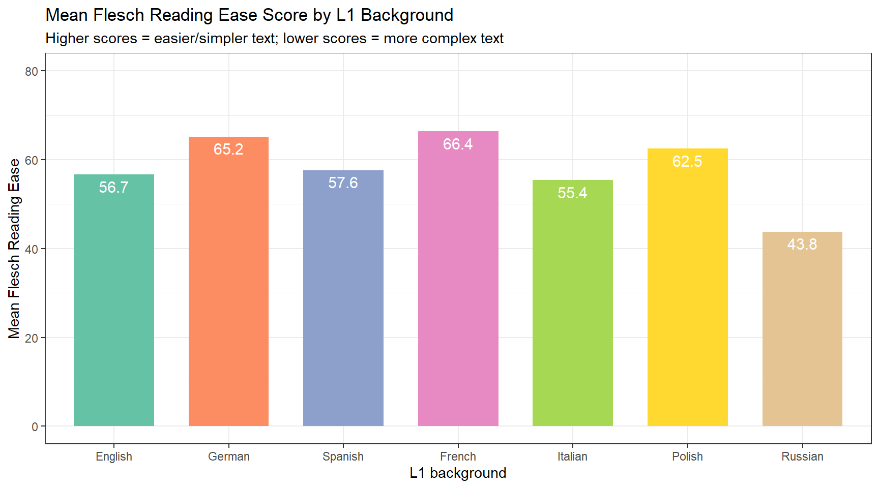
Readability

Readability measures quantify how easy or difficult a text is to read and comprehend. They are used in learner corpus research as indirect measures of writing quality and complexity. A text written by a highly proficient learner should be neither excessively simple nor unnecessarily complex. Here we focus on the Flesch Reading Ease score (Flesch 1948):

\[\text{Flesch} = 206.835 - (1.015 \times \text{ASL}) - \left(84.6 \times \frac{N_{\text{syllables}}}{N_{\text{words}}}\right)\]

where ASL is the average sentence length. Higher scores indicate easier text (shorter sentences, simpler words); scores below 30 indicate very difficult text, while scores above 70 indicate easy text. This creates a somewhat counter-intuitive situation for complexity research: higher proficiency does not necessarily mean higher Flesch scores — proficient writers often produce more complex (lower-scoring) text.

# Compute Flesch scores for each essay
ns1_read <- quanteda.textstats::textstat_readability(ns1_ess, measure = "Flesch")
ns2_read <- quanteda.textstats::textstat_readability(ns2_ess, measure = "Flesch")
de_read  <- quanteda.textstats::textstat_readability(de_ess,  measure = "Flesch")
es_read  <- quanteda.textstats::textstat_readability(es_ess,  measure = "Flesch")
fr_read  <- quanteda.textstats::textstat_readability(fr_ess,  measure = "Flesch")
it_read  <- quanteda.textstats::textstat_readability(it_ess,  measure = "Flesch")
pl_read  <- quanteda.textstats::textstat_readability(pl_ess,  measure = "Flesch")
ru_read  <- quanteda.textstats::textstat_readability(ru_ess,  measure = "Flesch")

# Combine into one table with L1 labels
read_all <- base::rbind(
  ns1_read, ns2_read, de_read, es_read, fr_read, it_read, pl_read, ru_read
) |>
  dplyr::mutate(
    l1 = c(
      rep("en", nrow(ns1_read) + nrow(ns2_read)),
      rep("de", nrow(de_read)), rep("es", nrow(es_read)),
      rep("fr", nrow(fr_read)), rep("it", nrow(it_read)),
      rep("pl", nrow(pl_read)), rep("ru", nrow(ru_read))
    ),
    l1 = factor(l1, levels = c("en", "de", "es", "fr", "it", "pl", "ru"))
  ) |>
  dplyr::group_by(l1) |>
  dplyr::summarise(Flesch = mean(Flesch, na.rm = TRUE), .groups = "drop")

read_all

# A tibble: 7 × 2
  l1    Flesch
  <fct>  <dbl>
1 en      56.7
2 de      65.2
3 es      57.6
4 fr      66.4
5 it      55.4
6 pl      62.5
7 ru      43.8

read_all |>
  ggplot(aes(x = l1, y = Flesch, label = round(Flesch, 1), fill = l1)) +
  geom_col(width = 0.7) +
  geom_text(vjust = 1.5, colour = "white", size = 4) +
  scale_x_discrete(labels = l1_labels) +
  scale_fill_brewer(palette = "Set2", guide = "none") +
  coord_cartesian(ylim = c(0, 80)) +
  theme_bw() +
  labs(
    title    = "Mean Flesch Reading Ease Score by L1 Background",
    subtitle = "Higher scores = easier/simpler text; lower scores = more complex text",
    x        = "L1 background",
    y        = "Mean Flesch Reading Ease"
  )

---

Check Your Understanding: Lexical Diversity and Readability

Q8. A researcher finds that Russian learners have the highest CTTR scores of all learner groups. Which interpretation is most warranted?

The CTTR scores prove that the Russian ICLE sub-corpus contains more essays than the other sub-corpora
Russian learners are definitively more proficient than all other learner groups
Russian learners use a more varied vocabulary per essay than other learner groups in this sample, though this could reflect essay length, topic treatment, or L1 transfer rather than proficiency alone
Russian is the most similar language to English, so transfer effects boost vocabulary diversity

---

Spelling Errors

Section Overview

What you’ll learn: How to use the hunspell package to detect words not found in a standard English dictionary, how to compute a normalised spelling error rate, and how to compare it across L1 groups

Key package: hunspell

Spelling accuracy is one of the most directly observable dimensions of L2 written proficiency. Although advanced learners generally make fewer spelling errors than beginners, systematic differences in error rates across L1 groups can reveal specific orthographic challenges associated with transfer from particular L1 writing systems. For example, learners whose L1 uses a transparent orthography (consistent grapheme-phoneme mappings) may transfer phonological spelling strategies to English that produce systematic errors (e.g. spelling based on pronunciation rather than convention).

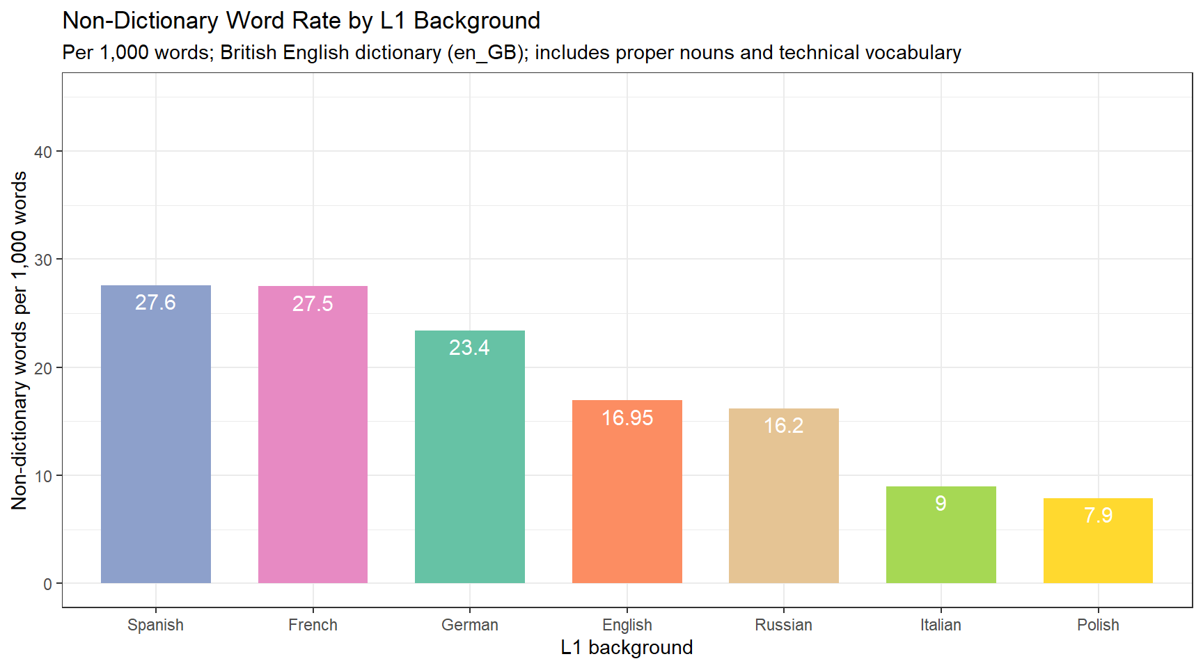
The hunspell package checks words against a dictionary and returns a list of words not found in it. We use the British English dictionary (en_GB) to match the LOCNESS corpus’s expected spelling norms.

Limitations of Dictionary-Based Spell Checking

Dictionary-based spell checking has several known limitations as a method for studying learner errors. It flags any word not in the dictionary — including proper nouns, technical vocabulary, abbreviations, and deliberate neologisms — as potential errors. It also misses real-word errors (e.g. their for there, form for from), which are spelled correctly but used in the wrong context. The counts here should therefore be interpreted as non-dictionary word rates rather than true spelling error rates.

# Inspect non-dictionary words in the first L1 essay
hunspell::hunspell(ns1_ess[1], dict = hunspell::dictionary("en_GB")) |>
  unlist() |>
  head(20)

[1] "dilema"     "UKs"        "incourage"  "conjestion" "Tourturing"

# Function: count non-dictionary words and total words per text set
spellStats <- function(texts, dict_code = "en_GB") {
  n_errors <- hunspell::hunspell(texts, dict = hunspell::dictionary(dict_code)) |>
    unlist() |>
    length()
  n_words  <- sum(tokenizers::count_words(texts))
  list(errors = n_errors, words = n_words)
}

# Apply to all text sets
spell_data <- list(
  en_ns1 = spellStats(ns1_ess), en_ns2 = spellStats(ns2_ess),
  de     = spellStats(de_ess),  es     = spellStats(es_ess),
  fr     = spellStats(fr_ess),  it     = spellStats(it_ess),
  pl     = spellStats(pl_ess),  ru     = spellStats(ru_ess)
)

# Build summary table: normalised error rate per 1,000 words
err_tb <- data.frame(
  l1     = c("en", "en", "de", "es", "fr", "it", "pl", "ru"),
  errors = sapply(spell_data, `[[`, "errors"),
  words  = sapply(spell_data, `[[`, "words")
) |>
  dplyr::mutate(freq = round(errors / words * 1000, 1)) |>
  dplyr::group_by(l1) |>
  dplyr::summarise(freq = mean(freq), .groups = "drop")

err_tb

# A tibble: 7 × 2
  l1     freq
  <chr> <dbl>
1 de     23.4
2 en     17.0
3 es     27.6
4 fr     27.5
5 it      9  
6 pl      7.9
7 ru     16.2

err_tb |>
  ggplot(aes(x = reorder(l1, -freq), y = freq, label = freq, fill = l1)) +
  geom_col(width = 0.7) +
  geom_text(vjust = 1.5, colour = "white", size = 4) +
  scale_x_discrete(labels = l1_labels) +
  scale_fill_brewer(palette = "Set2", guide = "none") +
  coord_cartesian(ylim = c(0, 45)) +
  theme_bw() +
  labs(
    title    = "Non-Dictionary Word Rate by L1 Background",
    subtitle = "Per 1,000 words; British English dictionary (en_GB); includes proper nouns and technical vocabulary",
    x        = "L1 background",
    y        = "Non-dictionary words per 1,000 words"
  )

---

Check Your Understanding: Spelling Errors

Q9. A researcher uses hunspell to count spelling errors in learner essays and finds that L1 English speakers have a higher non-dictionary word rate than some learner groups. How should this be interpreted?

This proves that L1 speakers make more spelling mistakes than learners
L1 speakers may use more proper nouns, colloquialisms, contractions, or domain-specific vocabulary not present in the standard dictionary — the hunspell count is not a pure spelling error count
The British English dictionary is biased against native speakers, so their errors are over-counted
L1 speakers intentionally write non-standard forms to demonstrate their proficiency

---

Summary and Best Practices

This tutorial has introduced seven corpus-based methods for analysing learner language in R. Working through these methods on the ICLE/LOCNESS data has illustrated both their practical application and their interpretive limits. A few overarching principles are worth emphasising:

Normalise before comparing. Raw frequency counts are almost always misleading when comparing across texts or corpora of different sizes. Always divide by total word count (or total token count) and express frequencies per 1,000 or per million words before drawing comparisons.

Use statistics to confirm visual impressions. Bar charts and box plots reveal patterns, but they cannot distinguish systematic differences from sampling variation. Fisher’s exact test (with Bonferroni correction for multiple comparisons) provides the inferential layer that transforms a visual observation into a defensible claim.

Triangulate across methods. No single measure fully captures the complexity of learner language. Sentence length, lexical diversity, POS-sequence frequencies, collocational patterns, readability, and spelling accuracy each illuminate a different dimension. Convergent evidence across multiple measures is more compelling than a single significant result.

Interpret measures in their context. Every measure discussed here has known limitations — TTR’s sensitivity to text length, Flesch’s insensitivity to syntactic complexity, hunspell’s conflation of errors with uncommon vocabulary. Always report these caveats alongside your findings.

Document your pre-processing. The results of learner corpus analyses are sensitive to cleaning decisions: which tags are stripped, how sentence boundaries are detected, which stopword list is used. Document every step in your code so that others (and your future self) can reproduce and evaluate your choices.

Citation and Session Info

Citation

Martin Schweinberger. 2026. Analysing Learner Language with R. The Language Technology and Data Analysis Laboratory (LADAL), The University of Queensland, Australia. url: https://ladal.edu.au/tutorials/learner_language/learner_language.html (Version 3.1.1), doi: 10.5281/zenodo.19332907.

@manual{martinschweinberger2026analysing,
  author       = {Martin Schweinberger},
  title        = {Analysing Learner Language with R},
  year         = {2026},
  note         = {https://ladal.edu.au/tutorials/learner_language/learner_language.html},
  organization = {The Language Technology and Data Analysis Laboratory (LADAL), The University of Queensland, Australia},
  edition      = {3.1.1}
  doi      = {10.5281/zenodo.19332907}
}

sessionInfo()

R version 4.4.2 (2024-10-31 ucrt)
Platform: x86_64-w64-mingw32/x64
Running under: Windows 11 x64 (build 26200)

Matrix products: default


locale:
[1] LC_COLLATE=English_United States.utf8 
[2] LC_CTYPE=English_United States.utf8   
[3] LC_MONETARY=English_United States.utf8
[4] LC_NUMERIC=C                          
[5] LC_TIME=English_United States.utf8    

time zone: Australia/Brisbane
tzcode source: internal

attached base packages:
[1] stats     graphics  grDevices datasets  utils     methods   base     

other attached packages:
 [1] slam_0.1-55               Matrix_1.7-2             
 [3] tokenizers_0.3.0          wordcloud2_0.2.1         
 [5] hunspell_3.0.5            stringi_1.8.7            
 [7] koRpus_0.13-8             sylly_0.1-6              
 [9] quanteda.textplots_0.95   quanteda.textstats_0.97.2
[11] quanteda_4.2.0            udpipe_0.8.11            
[13] tidytext_0.4.3            flextable_0.9.11         
[15] lubridate_1.9.4           forcats_1.0.0            
[17] stringr_1.6.0             dplyr_1.2.0              
[19] purrr_1.2.1               readr_2.1.5              
[21] tidyr_1.3.2               tibble_3.3.1             
[23] ggplot2_4.0.2             tidyverse_2.0.0          
[25] checkdown_0.0.13         

loaded via a namespace (and not attached):
 [1] tidyselect_1.2.1        viridisLite_0.4.2       farver_2.1.2           
 [4] S7_0.2.1                fastmap_1.2.0           fontquiver_0.2.1       
 [7] janeaustenr_1.0.0       digest_0.6.39           timechange_0.3.0       
[10] lifecycle_1.0.5         magrittr_2.0.4          compiler_4.4.2         
[13] rlang_1.1.7             tools_4.4.2             utf8_1.2.6             
[16] yaml_2.3.10             sna_2.8                 data.table_1.17.0      
[19] knitr_1.51              askpass_1.2.1           labeling_0.4.3         
[22] stopwords_2.3           htmlwidgets_1.6.4       here_1.0.2             
[25] xml2_1.3.6              RColorBrewer_1.1-3      withr_3.0.2            
[28] grid_4.4.2              gdtools_0.5.0           scales_1.4.0           
[31] cli_3.6.5               rmarkdown_2.30          ragg_1.5.1             
[34] generics_0.1.4          rstudioapi_0.17.1       tzdb_0.5.0             
[37] commonmark_2.0.0        network_1.19.0          BiocManager_1.30.27    
[40] vctrs_0.7.2             jsonlite_2.0.0          fontBitstreamVera_0.1.1
[43] litedown_0.9            ISOcodes_2024.02.12     hms_1.1.4              
[46] patchwork_1.3.0         ggrepel_0.9.8           systemfonts_1.3.1      
[49] glue_1.8.0              statnet.common_4.11.0   codetools_0.2-20       
[52] gtable_0.3.6            pillar_1.11.1           htmltools_0.5.9        
[55] openssl_2.3.2           R6_2.6.1                textshaping_1.0.0      
[58] rprojroot_2.1.1         evaluate_1.0.5          lattice_0.22-6         
[61] markdown_2.0            SnowballC_0.7.1         renv_1.1.7             
[64] fontLiberation_0.1.0    Rcpp_1.1.1              zip_2.3.2              
[67] uuid_1.2-1              fastmatch_1.1-8         coda_0.19-4.1          
[70] nsyllable_1.0.1         officer_0.7.3           xfun_0.56              
[73] pkgconfig_2.0.3        

AI Transparency Statement

This tutorial was re-developed with the assistance of Claude (claude.ai), a large language model created by Anthropic. Claude was used to help revise the tutorial text, structure the instructional content, generate the R code examples, and write the checkdown quiz questions and feedback strings. All content was reviewed, edited, and approved by the author (Martin Schweinberger), who takes full responsibility for the accuracy and pedagogical appropriateness of the material. The use of AI assistance is disclosed here in the interest of transparency and in accordance with emerging best practices for AI-assisted academic content creation.

Back to top

Back to LADAL home

References

Daller, Helmut, James Milton, Jeanine Treffers-Daller, et al. 2007. Modelling and Assessing Vocabulary Knowledge. Vol. 10. Cambridge University Press Cambridge.

Flesch, Rudolph. 1948. “A New Readability Yardstick.” Journal of Applied Psychology 32 (3): 221–33. https://doi.org/https://doi.org/10.1037/h0057532.

Gilquin, Gaëtanelle, and S Granger. 2015. “From Design to Collection of Learner Corpora.” The Cambridge Handbook of Learner Corpus Research 3 (1): 9–34.

Granger, Sylviane. 2009. “The Contribution of Learner Corpora to Second Language Acquisition and Foreign Language Teaching.” Corpora and Language Teaching 33: 13–32.

Granger, Sylviane, Estelle Dagneaux, Fanny Meunier, Magali Paquot, et al. 1993. “The International Corpus of Learner English.” English Language Corpora: Design, Analysis and Exploitation, 57–71.

Granger, Sylviane, Carol Sanders, and Ulla Connor. 2005. “LOCNESS: Louvain Corpus of Native English Essays.” Louvain-la-Neuve, Belgium: Centre for English Corpus Linguistics (CECL), Université catholique de Louvain.

Kyle, Kristopher, and Scott A Crossley. 2018. “Measuring Syntactic Complexity in L2 Writing Using Fine-Grained Clausal and Phrasal Indices.” The Modern Language Journal 102 (2): 333–49.

Lindquist, Hans. 2009. Corpus Linguistics and the Description of English. Vol. 104. Edinburgh: Edinburgh University Press.

Nesselhauf, Nadja. 2005. “Structural and Functional Properties of Collocations in English. A Corpus Study of Lexical and Pragmatic Constraints on Lexical Co-Occurrence.” International Journal of Corpus Linguistics 10 (2): 266–70.

Selinker, Larry, Merrill Swain, and Guy Dumas. 1975. “The Interlanguage Hypothesis Extended to Children 1.” Language Learning 25 (1): 139–52.