R Markdown and Quarto: Creating Reproducible Documents

Author

Martin Schweinberger

Published

2026

Great Court, The University of Queensland

Introduction

This tutorial introduces R Markdown and Quarto as tools for combining code, output, and narrative text in a single, dynamic, and fully reproducible document. Whether you are writing a corpus analysis report, a phonetics study, or a data science notebook, these tools allow you to weave together your R code, its output, and your prose explanation into a polished, shareable document.

The tutorial is aimed at beginners and intermediate R users in the humanities and social sciences. It covers the full workflow: understanding what R Markdown and Quarto are and how they differ, learning Markdown syntax, configuring YAML headers, controlling code chunk behaviour, producing multiple output formats, and using Quarto’s advanced features such as callout blocks, cross-references, citations, and project-level configuration.

By the end of this tutorial you will be able to:

Create a reproducible R Markdown or Quarto document from scratch
Write well-structured Markdown prose with headings, lists, tables, and figures
Control how code chunks are displayed and executed
Export your work as HTML, PDF, Word, or a presentation
Use Quarto-specific features: callouts, cross-references, freeze, and _quarto.yml
Manage citations and bibliographies with BibTeX

Prerequisite Knowledge

Before working through this tutorial, you should be familiar with:

Basic R syntax and RStudio (Getting Started with R)
Saving and loading files in R (Loading, Saving, and Generating Data in R)

Citation

Martin Schweinberger. 2026. R Markdown and Quarto: Creating Reproducible Documents. The Language Technology and Data Analysis Laboratory (LADAL), The University of Queensland, Australia. url: https://ladal.edu.au/tutorials/notebooks/notebooks.html (Version 3.1.1). doi: 10.5281/zenodo.19332919.

Setup

Installing Packages

Code

# Run once — comment out after installation
install.packages("rmarkdown")
install.packages("knitr")
install.packages("tidyverse")
install.packages("flextable")
install.packages("kableExtra")
install.packages("bookdown")    # for cross-references in R Markdown
# Quarto is installed separately from https://quarto.org/docs/get-started/

Loading Packages

Code

library(rmarkdown)
library(knitr)
library(tidyverse)
library(flextable)
klippy::klippy()

What Are R Markdown and Quarto?

Section Overview

What you will learn: What R Markdown and Quarto are; why reproducible documents matter; and how these tools fit into a modern research workflow

The Problem They Solve

A typical research workflow involves several disconnected steps: running R code in a script, copying results into a Word document, inserting figures manually, and then updating everything again when the data changes. This workflow is fragile — a change in the data means re-running the code, re-copying the numbers, and re-inserting the figures, with every step introducing the risk of inconsistency.

R Markdown and Quarto solve this by integrating code, output, and prose in a single source document. When you render the document, the code runs, the output is inserted automatically, and the prose and results are always in sync. The document is reproducible: anyone with the source file and data can re-render it and obtain exactly the same output.

R Markdown

R Markdown was introduced by the knitr package (Xie 2017) and formalised in the rmarkdown package (Allaire et al. 2023). An R Markdown document (.Rmd) combines:

A YAML header specifying document metadata and output format
Markdown prose for narrative text
R code chunks that are executed when the document is rendered

R Markdown documents are rendered by knitr (which executes the R code and weaves the output into the document) followed by Pandoc (which converts the resulting Markdown into the target output format — HTML, PDF, Word, etc.).

Quarto

Quarto is the next-generation publishing system developed by Posit (formerly RStudio). A Quarto document (.qmd) uses the same Markdown + code chunk approach as R Markdown, but with several important advances:

Language-agnostic: supports R, Python, Julia, and Observable JS in the same document
Unified syntax: chunk options use #| comments rather than chunk header parameters
Richer output features: built-in callout blocks, cross-references, layouts, and theming
Project system: _quarto.yml configures entire websites, books, or presentations
Better defaults: produces cleaner HTML and PDF output out of the box

For new projects, Quarto is recommended. R Markdown remains fully supported and is still widely used. This tutorial covers both.

R Markdown vs. Quarto

Section Overview

What you will learn: How R Markdown and Quarto differ in syntax, features, and workflow; and when to use each

Feature	R Markdown	Quarto
File extension	`.Rmd`	`.qmd`
Engine	`knitr` → Pandoc	`knitr` or `jupyter` → Pandoc
Language support	Primarily R; Python via `reticulate`	R, Python, Julia, Observable JS
Chunk options syntax	Inside chunk header: `{r label, echo=FALSE}`	`#\|` comments inside chunk: `#\| echo: false`
YAML location	Document YAML header only	Document YAML + `_quarto.yml` project file
Callout blocks	Via `rmdformats` or custom CSS	Built-in (`.callout-note`, `.callout-warning`, etc.)
Cross-references	Via `bookdown` package	Built-in `@fig-`, `@tbl-`, `@sec-` syntax
Project system	Limited — manual setup	`_quarto.yml` for websites, books, presentations
Slides	`ioslides`, `Slidy`, `Beamer` (PDF)	Reveal.js (HTML); Beamer (PDF); PowerPoint
Books / websites	`bookdown`, `blogdown`, `distill`	Built-in `quarto render` project commands
Inline code	`` `r expr` ``	`` `r .QuartoInlineRender(expr)` `` or `` `r expr` ``
Freeze / caching	Via `knitr` cache	`freeze: auto` in `_quarto.yml`
Maintained by	Posit / community	Posit
When to use	Existing `.Rmd` projects; R-only workflows	New projects; multi-language; websites; books

Which Should I Use?

Use R Markdown if you are working on an existing .Rmd project, or if you need a package that is R Markdown-specific (e.g. blogdown, bookdown)
Use Quarto for all new projects — it is more powerful, better maintained, and handles multi-language workflows elegantly
Both render to the same output formats via Pandoc, so skills transfer directly between them

Creating Your First Document

Section Overview

What you will learn: How to create a new R Markdown or Quarto document in RStudio; what the basic structure looks like; and how to render it

In RStudio

R Markdown: Go to File → New File → R Markdown. Choose the output format (HTML is the default) and click OK. RStudio creates a template .Rmd file with a YAML header, some sample text, and a few code chunks.

Quarto: Go to File → New File → Quarto Document. Again choose your output format and click Create. RStudio creates a template .qmd file.

Basic Structure

Both document types share the same three-part structure:

---
YAML header
---

Markdown prose

` ``{r}
# R code chunk
` ``

Rendering

R Markdown: Click the Knit button in RStudio (or run rmarkdown::render("file.Rmd") in the console).

Quarto: Click the Render button in RStudio (or run quarto render file.qmd in the terminal).

Both processes: execute all code chunks → weave output into the document → convert to the target format via Pandoc.

Keyboard Shortcut

Ctrl+Shift+K (Windows/Linux) or Cmd+Shift+K (Mac) renders the current document in RStudio — for both R Markdown and Quarto.

YAML Headers

Section Overview

What you will learn: What YAML is; the most important YAML fields for R Markdown and Quarto; how to configure output formats, themes, and table of contents; and how Quarto’s YAML extends R Markdown’s

What Is YAML?

YAML (Yet Another Markup Language) is a human-readable data serialisation format used to store configuration. In R Markdown and Quarto, the YAML header sits between two sets of --- at the top of the document and controls metadata (title, author, date) and rendering options (output format, theme, table of contents).

YAML is indentation-sensitive — use spaces, not tabs, and be consistent with nesting.

R Markdown YAML

A minimal R Markdown YAML header:

title: "My Analysis"
author: "Martin Schweinberger"
date: "2026-03-10"
output: html_document

A fully configured HTML output header:

title: "Corpus Frequency Analysis"
author: "Martin Schweinberger"
date: "YYYY-MM-DD   # use Sys.Date() in practice"
output:
  html_document:
    toc: true
    toc_depth: 3
    toc_float: true
    number_sections: true
    theme: cosmo
    highlight: tango
    code_folding: show
    df_print: paged
bibliography: references.bib
csl: unified-style-linguistics.csl

Multiple output formats in one document:

title: "My Document"
output:
  html_document:
    toc: true
  pdf_document:
    toc: true
  word_document:
    reference_docx: template.docx

Field	Description
`title`	Document title — appears as the main heading
`author`	Author name(s) — can be a list
`date`	Date string or inline R expression e.g. `` `r Sys.Date()` ``
`output`	Output format: `html_document`, `pdf_document`, `word_document`, etc.
`toc`	Include table of contents (`true`/`false`)
`toc_depth`	Depth of headings included in the ToC (default 3)
`toc_float`	Float the ToC in the sidebar (HTML only)
`number_sections`	Auto-number sections (`true`/`false`)
`theme`	Bootstrap theme for HTML (cosmo, flatly, journal, etc.)
`highlight`	Syntax highlighting style (tango, pygments, kate, etc.)
`code_folding`	Show/hide code (`show`, `hide`, `none`)
`df_print`	How data frames are printed (`default`, `kable`, `tibble`, `paged`)
`bibliography`	Path to `.bib` bibliography file
`csl`	Citation style language file for reference formatting
`params`	Parameterised report inputs — see Parameterised Reports section

Quarto YAML

Quarto’s YAML uses nested format: keys rather than output:, and adds many new fields:

title: "Corpus Frequency Analysis"
author:
  - name: "Martin Schweinberger"
    affiliation: "The University of Queensland"
    email: "m.schweinberger@uq.edu.au"
date: last-modified
date-format: "DD MMMM YYYY"
format:
  html:
    toc: true
    toc-depth: 4
    toc-title: "Contents"
    toc-location: left
    number-sections: true
    number-depth: 3
    code-fold: show
    code-tools: true
    code-line-numbers: true
    theme: cosmo
    highlight-style: tango
    embed-resources: true
    smooth-scroll: true
    citations-hover: true
    footnotes-hover: true
  pdf:
    documentclass: article
    geometry: margin=2.5cm
    toc: true
  docx:
    reference-doc: template.docx
execute:
  echo: true
  warning: false
  message: false
  cache: false
bibliography: references.bib
csl: unified-style-linguistics.csl
lang: en-GB

Field	Description
`title`	Document title
`author`	Can be a list with `name`, `affiliation`, `email`, `orcid`
`date: last-modified`	Automatically set to the file's last-modified date
`date-format`	Date display format using `dayjs` tokens
`format: html:`	HTML output options — nested under `format: html:`
`toc-location`	Position of ToC: `left`, `right`, `body`
`code-fold`	Code folding: `show`, `hide`, `true`, `false`
`code-tools`	Show a toolbar to copy code or view source
`code-line-numbers`	Add line numbers to code blocks
`embed-resources`	Bundle all dependencies into a single self-contained HTML file
`smooth-scroll`	Enable smooth scrolling between sections
`citations-hover`	Show citation details on hover
`execute:`	Global chunk execution defaults — applies to all chunks
`execute: cache`	Cache all chunk outputs to speed up re-rendering
`lang`	Document language for hyphenation and accessibility
`bibliography`	Path to `.bib` file
`csl`	Citation style language file

Code Chunks

Section Overview

What you will learn: How to insert and label code chunks; how to control their execution, display, and output with chunk options; and how R Markdown and Quarto chunk syntax differ

Inserting a Code Chunk

Keyboard shortcut: Ctrl+Alt+I (Windows/Linux) or Cmd+Option+I (Mac) inserts a new code chunk in RStudio.

R Markdown syntax — options go in the chunk header:

` ` `{r my-chunk-label, echo=TRUE, message=FALSE, warning=FALSE}
# R code here
` ` `

Quarto syntax — options go inside the chunk as #| comments:

` ` `{r}
#| label: my-chunk-label
#| echo: true
#| message: false
#| warning: false
# R code here
` ` `

Both syntaxes are valid in Quarto, but the #| style is preferred because it is language-agnostic (the same syntax works for Python, Julia, etc.) and keeps chunk options inside the chunk where they are easier to see.

Chunk Option Reference

Option	R Markdown	Quarto	Effect
`label`	`label`	`label`	Unique chunk identifier (required for cross-refs and caching)
`echo`	`echo`	`echo`	`true` show code; `false` hide code; `fenced` show with delimiters
`eval`	`eval`	`eval`	`true` run the chunk; `false` skip execution entirely
`include`	`include`	`include`	`false` run but suppress ALL output including code, results, messages
`message`	`message`	`message`	`false` suppress package messages (e.g. `library()` output)
`warning`	`warning`	`warning`	`false` suppress warnings
`error`	`error`	`error`	`true` show errors instead of stopping render
`results`	`results`	`results`	`hide` suppress printed output; `asis` pass raw HTML/Markdown through
`output`	—	`output`	Quarto alias for `results`
`fig.height` / `fig-height`	`fig.height`	`fig-height`	Plot height in inches (default 5)
`fig.width` / `fig-width`	`fig.width`	`fig-width`	Plot width in inches (default 7)
`fig.cap` / `fig-cap`	`fig.cap`	`fig-cap`	Figure caption string
`fig.align` / `fig-align`	`fig.align`	`fig-align`	`left`, `center`, `right`
`fig.show` / `fig-show`	`fig.show`	`fig-show`	`hold` collect all plots; `hide` suppress plots
`out.width` / `out-width`	`out.width`	`out-width`	Scale output width e.g. `'80%'` or `'400px'`
`cache`	`cache`	`cache`	`true` cache chunk output to disk
`dependson`	`dependson`	`dependson`	Labels of chunks this chunk depends on for cache invalidation
`child`	`child`	`child`	Path to a child `.Rmd`/`.qmd` to include
`code`	`code`	`code`	Override code displayed in the chunk
`collapse`	`collapse`	`collapse`	`true` collapse code and output into one block

Practical Examples

Show code but hide output:

` ``{r}
#| echo: true
#| output: false
summary(mtcars)
` ``

Hide code, show only the plot:

` ``{r}
#| echo: false
#| fig-height: 5
#| fig-width: 7
#| fig-cap: "Distribution of word lengths"
#| fig-align: center
hist(nchar(words))
` ``

Run chunk but suppress everything (useful for setup):

` ``{r}
#| include: false
library(tidyverse)
library(flextable)
` ``

Display a figure at 80% page width, centred:

` ``{r}
#| out-width: "80%"
#| fig-align: center
#| fig-cap: "Vowel space of RP speakers"
plot(vowel_chart)
` ``

Cache an expensive computation:

` ``{r}
#| label: heavy-model
#| cache: true
model <- lmer(RT ~ Frequency + (1|Subject), data = lexdec)
` ``

Global Chunk Options

Setting options individually on every chunk is tedious. Use a setup chunk to set defaults for the whole document.

R Markdown:

` ``{r setup, include=FALSE}
knitr::opts_chunk$set(
  echo    = TRUE,
  message = FALSE,
  warning = FALSE,
  fig.height = 5,
  fig.width  = 7,
  fig.align  = "center"
)
` ``

Quarto — set in the YAML execute: block instead:

execute:
  echo: true
  message: false
  warning: false

Figure defaults in Quarto go under fig-:

format:
  html:
    fig-height: 5
    fig-width: 7
    fig-align: center

Inline Code

Inline code embeds a computed value directly in prose without a separate code chunk:

R Markdown: write a backtick followed immediately by r, then a space, your expression, and a closing backtick — directly in prose. When rendered, the expression is replaced by its computed value — e.g. The corpus contains 4,572 tokens.

Quarto: the equivalent syntax is a backtick followed by {r}, a space, your expression, and a closing backtick — placed in prose. The older R Markdown syntax also works in Quarto.

Inline code is rendered inline — the expression is replaced with its value in the output. This ensures numbers in your prose always match your data.

Markdown Syntax Reference

Section Overview

What you will learn: The full Markdown syntax supported by R Markdown and Quarto, from basic formatting to advanced features like footnotes, math, diagrams, and HTML

Headings

Command:

# Heading 1
## Heading 2
### Heading 3
#### Heading 4
##### Heading 5
###### Heading 6

Rendered:

Heading 1

Heading 2

Heading 3

Heading 4

Heading 5

Heading 6

Headings can carry a custom ID for cross-referencing and linking:

## Results {#sec-results}

And can carry Quarto classes to suppress numbering:

## Appendix {.unnumbered}

Emphasis

Command:

*italic*    _italic_
**bold**    __bold__
***bold and italic***
~~strikethrough~~

Rendered:

italic / italic · bold / bold · bold and italic · ~~strikethrough~~

Quarto also supports:

H~2~O          (subscript)
E = mc^2^      (superscript)
[mark]{.mark}  (highlight — requires appropriate CSS)

Rendered: H₂O · E = mc² · mark

Lists

Unordered List

- Item 1
- Item 2
  - Subitem 2.1
  - Subitem 2.2
- Item 3

Item 1
Item 2
- Subitem 2.1
- Subitem 2.2
Item 3

Ordered List

1. First item
2. Second item
3. Third item
   1. Subitem 3.1
   2. Subitem 3.2

First item
Second item
Third item
1. Subitem 3.1
2. Subitem 3.2

Task Lists

- [x] Completed task
- [ ] Incomplete task
- [ ] Another task
  - [x] Completed subtask
  - [ ] Pending subtask

Definition Lists

Monophthong
: A vowel with a single, stable tongue position during production.

Diphthong
: A vowel that involves a glide from one tongue position to another.

Formant
: A resonant frequency band produced by the vocal tract shape.

Monophthong: A vowel with a single, stable tongue position during production.
Diphthong: A vowel that involves a glide from one tongue position to another.
Formant: A resonant frequency band produced by the vocal tract shape.

Links

[LADAL](https://ladal.edu.au)                    # external link
[Introduction](#intro)                            # internal anchor link
[Schweinberger 2026](references.html#ref-sch26)  # link to reference
<m.schweinberger@uq.edu.au>                       # auto-linked email

Rendered: LADAL · Introduction · m.schweinberger@uq.edu.au

Images

Basic image:

![Alt text](/images/vowelchartrp.png)

Image with width and alignment (Quarto/Pandoc attribute syntax):

![Vowel chart of RP](/images/vowelchartrp.png){width=60% fig-align="center"}

Floating image (HTML inline style):

![](/images/gy_chili.png){ width=15% style="float:right; padding:10px" }

Image with a cross-referenceable label:

![Vowel chart of RP](/images/vowelchartrp.png){#fig-vc width=70%}

See @fig-vc for the vowel chart.

Two images side by side using Quarto layout:

::: {layout-ncol=2}
![Left panel](/images/fig1.png){#fig-left}
![Right panel](/images/fig2.png){#fig-right}
:::

Blockquotes

> This is a blockquote.
>
> Spanning multiple paragraphs.
>
> > This is a nested blockquote.

This is a blockquote.

Spanning multiple paragraphs.

This is a nested blockquote.

Blockquotes with attribution:

> The limits of my language mean the limits of my world.
>
> — Ludwig Wittgenstein, *Tractatus Logico-Philosophicus* (1921)

The limits of my language mean the limits of my world.

— Ludwig Wittgenstein, Tractatus Logico-Philosophicus (1921)

Code

Inline Code

Use `read.table()` to load tab-delimited files.

Use read.table() to load tab-delimited files.

Code Blocks

Fenced code blocks with language tags produce syntax highlighting:

```r
corpus <- readLines("corpus.txt")
tokens <- unlist(strsplit(corpus, "\\s+"))
```

corpus <- readLines("corpus.txt")
tokens <- unlist(strsplit(corpus, "\\s+"))

Supported language tags include: r, python, bash, markdown, yaml, json, html, latex, praat, and many more.

Tables

Basic Markdown Table

| Vowel | IPA | F1 (Hz) | F2 (Hz) |
|-------|-----|---------|---------|
| heed  | iː  | 276     | 2338    |
| hid   | ɪ   | 393     | 2174    |
| head  | e   | 600     | 1926    |
| had   | æ   | 916     | 1473    |

Vowel	IPA	F1 (Hz)	F2 (Hz)
heed	iː	276	2338
hid	ɪ	393	2174
head	e	600	1926
had	æ	916	1473

Column Alignment

| Left     | Centre   | Right    |
|:---------|:--------:|---------:|
| text     | text     | 1,234    |
| text     | text     | 5,678    |

Left	Centre	Right
text	text	1,234
text	text	5,678

For production tables — sortable columns, striped rows, captions, cross-references — use flextable() or knitr::kable() in a code chunk rather than raw Markdown tables.

Footnotes

Formants are resonant frequencies of the vocal tract.[^1]

[^1]: For a thorough introduction to formant analysis see Johnson (2003).

Formants are resonant frequencies of the vocal tract.¹

Inline footnotes (Quarto/Pandoc):

Formants are resonant frequencies of the vocal tract.^[For a thorough introduction see Johnson (2003).]

Math Expressions

Inline LaTeX math:

The polarity ratio is $P = \frac{n_+}{n_-}$.

The polarity ratio is $P = \frac{n_+}{n_-}$.

Display (block) math:

$$
F_{\text{Lobanov}} = \frac{F - \bar{F}_{\text{speaker}}}{SD_{F,\text{speaker}}}
$$

\[ F_{\text{Lobanov}} = \frac{F - \bar{F}_{\text{speaker}}}{SD_{F,\text{speaker}}} \]

Mermaid Diagrams

Quarto supports Mermaid diagrams natively with no extra packages:

```{mermaid}
graph TD
    A[Raw audio] --> B[Praat formant extraction]
    B --> C[Tab-delimited .txt file]
    C --> D[Load in R]
    D --> E[Normalisation]
    E --> F[Vowel chart]
```

graph TD
    A[Raw audio] --> B[Praat formant extraction]
    B --> C[Tab-delimited .txt file]
    C --> D[Load in R]
    D --> E[Normalisation]
    E --> F[Vowel chart]

Other diagram types: flowchart, sequenceDiagram, gantt, classDiagram, stateDiagram, erDiagram, pie.

HTML Elements

Raw HTML passes through directly in both R Markdown and Quarto HTML output.

Expandable section:

<details>
  <summary>Click to expand: full model output</summary>
  Content hidden until expanded. Useful for supplementary material.
</details>

Click to expand: full model output

Content hidden until expanded. Useful for supplementary material.

Coloured span (requires inline CSS):

<span style="color: #E67E22; font-weight: bold;">Important term</span>

Important term

Keyboard key styling:

Press <kbd>Ctrl</kbd>+<kbd>Shift</kbd>+<kbd>K</kbd> to render.

Press Ctrl+Shift+K to render.

Escaping Special Characters

Backslash escapes Markdown special characters:

\*not italic\*   \`not code\`   \# not a heading   \[not a link\]

*not italic* · `not code` · # not a heading · [not a link]

Horizontal Rules

---
***
___

All three produce a horizontal rule:

Emojis

:smile: :+1: :sparkles: :books: :bar_chart:

:smile: :+1: :sparkles: :books: :bar_chart:

(Requires emoji extension or appropriate Pandoc version — works in Quarto HTML by default.)

Output Formats

Section Overview

What you will learn: How to render R Markdown and Quarto documents to HTML, PDF, Word, and presentation formats; what options are available for each; and how to choose the right format for your audience

HTML

HTML is the richest output format — it supports interactive widgets, floating tables of contents, collapsible code, hover citations, and smooth scrolling. It is the recommended format for sharing analysis online or via email.

R Markdown:

output:
  html_document:
    toc: true
    toc_float: true
    theme: cosmo
    code_folding: show
    df_print: paged

Quarto:

format:
  html:
    toc: true
    toc-location: left
    theme: cosmo
    code-fold: show
    embed-resources: true   # self-contained single file

embed-resources: true

By default, Quarto HTML output references external libraries (Bootstrap, highlight.js, etc.) via relative paths. Setting embed-resources: true bundles everything into a single .html file — ideal for sharing by email or uploading to a repository without worrying about broken relative paths.

PDF

PDF output requires a LaTeX distribution. The recommended option is TinyTeX, which can be installed from R:

Code

install.packages("tinytex")
tinytex::install_tinytex()

R Markdown:

output:
  pdf_document:
    toc: true
    number_sections: true
    latex_engine: xelatex   # for Unicode and custom fonts
    keep_tex: true          # keep the intermediate .tex file

Quarto:

format:
  pdf:
    documentclass: article
    geometry: margin=2.5cm
    toc: true
    number-sections: true
    latex-engine: xelatex
    include-in-header: preamble.tex   # custom LaTeX preamble

PDF and Unicode

If your document contains IPA symbols, non-Latin scripts, or special characters, use latex_engine: xelatex (R Markdown) or latex-engine: xelatex (Quarto). The default pdflatex engine does not support Unicode. Also ensure your fonts support the required character ranges.

Word (.docx)

Word output is useful when collaborators need to add track-changes comments or when a journal requires .docx submission.

R Markdown:

output:
  word_document:
    toc: true
    reference_docx: template.docx   # custom styles template

Quarto:

format:
  docx:
    toc: true
    reference-doc: template.docx
    highlight-style: github

To create a Word template: render a document to .docx, open it in Word, modify the Heading 1, Body Text, Code, and Caption styles to match your requirements, save it, and point reference_docx/reference-doc at it.

Presentations

Quarto Reveal.js (HTML Slides)

Reveal.js is Quarto’s primary presentation format — fully interactive, browser-based slides:

format:
  revealjs:
    theme: simple         # default, simple, sky, moon, serif, solarized
    slide-number: true
    chalkboard: true      # interactive drawing on slides
    incremental: true     # bullet points appear one at a time
    footer: "LADAL — ladal.edu.au"
    logo: /images/uq1.jpg
    transition: slide     # none, fade, slide, convex, concave, zoom
    background-transition: fade

In a Reveal.js document, each ## heading starts a new slide, and --- creates a slide without a heading. Columns are created with:

:::: {.columns}
::: {.column width="50%"}
Left column content
:::
::: {.column width="50%"}
Right column content
:::
::::

Beamer (PDF Slides)

format:
  beamer:
    theme: Madrid
    colortheme: dolphin
    fonttheme: structurebold
    slide-level: 2

PowerPoint

format:
  pptx:
    reference-doc: template.pptx

R Markdown Presentations

output:
  ioslides_presentation:
    widescreen: true
    smaller: true
  slidy_presentation:
    footer: "LADAL"
  beamer_presentation:
    theme: Madrid

Format	Best for	R Markdown	Quarto
HTML (`html_document`/`html`)	Online sharing; interactive outputs; most feature-rich	✓	✓
PDF (`pdf_document`/`pdf`)	Print; journal submission; formal reports	✓	✓
Word (`word_document`/`docx`)	Collaboration with track changes; journal .docx submission	✓	✓
Reveal.js (`revealjs`)	Interactive HTML presentations with code output	—	✓
Beamer (`beamer`)	PDF presentations; conference talks with LaTeX typesetting	✓	✓
PowerPoint (`pptx`)	PowerPoint-compatible presentations for non-R users	✓	✓
ioslides / Slidy	Simple HTML presentations (R Markdown only)	✓	—

Quarto-Specific Features

Section Overview

What you will learn: Quarto’s built-in callout blocks; multi-column and panel layouts; tabsets; the freeze execution option; and the _quarto.yml project configuration file

Callout Blocks

Callout blocks draw attention to notes, tips, warnings, and important information. They are a Quarto native feature — no extra packages or CSS required.

::: {.callout-note}
## Note title
This is a note callout — used for supplementary information.
:::

::: {.callout-tip}
## Tip title
This is a tip callout — used for best practices and shortcuts.
:::

::: {.callout-warning}
## Warning title
This is a warning callout — used for common mistakes and pitfalls.
:::

::: {.callout-important}
## Important title
This is an important callout — used for critical information.
:::

::: {.callout-caution}
## Caution title
This is a caution callout — used for potential issues requiring care.
:::

Rendered:

Note title

This is a note callout — used for supplementary information.

Tip title

This is a tip callout — used for best practices and shortcuts.

Warning title

This is a warning callout — used for common mistakes and pitfalls.

Important title

This is an important callout — used for critical information.

Caution title

This is a caution callout — used for potential issues requiring care.

Callouts can be collapsed by default:

::: {.callout-note collapse="true"}
## Expandable note
This content is hidden until the reader clicks the heading.
:::

Expandable note

This content is hidden until the reader clicks the heading.

Callouts without a title:

::: {.callout-tip appearance="simple"}
A quick tip with no header.
:::

A quick tip with no header.

Multi-Column Layouts

Two-Column Body Text

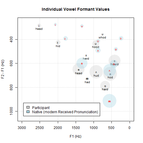
:::: {.columns}
::: {.column width="60%"}
**Main analysis**

The vowel chart reveals that the learner's /iː/ is more centralised
than the RP target, with F2 approximately 200 Hz lower than expected.
:::
::: {.column width="40%"}
**Key finding**

- /iː/ centralised
- /ɔː/ raised
- /æ/ raised and backed
:::
::::

Main analysis

The vowel chart reveals that the learner’s /iː/ is more centralised than the RP target, with F2 approximately 200 Hz lower than expected.

Key finding

/iː/ centralised
/ɔː/ raised
/æ/ raised and backed

Figure Layouts

Place two figures side by side with independent captions and cross-reference labels:

::: {#fig-comparison layout-ncol=2}

![Raw Hz](/images/plot_raw.png){#fig-raw}

![Lobanov-normalised](/images/plot_lob.png){#fig-lob}

Vowel space before (left) and after (right) Lobanov normalisation.
:::

See @fig-comparison for the comparison, or specifically @fig-raw for raw Hz values.

Layout options: layout-ncol, layout-nrow, or a custom layout matrix:

::: {layout="[[1,1],[1]]"}
![Top left](/images/a.png)
![Top right](/images/b.png)
![Full width bottom](/images/c.png)
:::

Tabsets

Tabsets allow multiple versions of content in the same space — useful for showing results under different conditions, or code in multiple languages:

::: {.panel-tabset}
## Raw Hz

Content for the raw Hz tab.

## Lobanov

Content for the Lobanov normalisation tab.

## Nearey

Content for the Nearey normalisation tab.
:::

Content for the raw Hz tab.

Content for the Lobanov normalisation tab.

Content for the Nearey normalisation tab.

The `freeze` Option

Rendering a Quarto document re-executes all code chunks. For documents with long-running computations (large models, web scraping), this is expensive. The freeze option caches executed output so that chunks are only re-run when their code changes.

In _quarto.yml (applies to all documents in the project):

execute:
  freeze: auto   # re-execute only when source code changes

In an individual document’s YAML:

execute:
  freeze: true   # never re-execute — always use cached output

Cached output is stored in the _freeze/ directory. Commit this directory to version control so collaborators can render the document without re-running expensive computations.

The `_quarto.yml` Project File

A _quarto.yml file in the root of a project configures all documents simultaneously. This is the key advantage of the Quarto project system over R Markdown.

Website Project

project:
  type: website
  output-dir: docs          # rendered output goes here (for GitHub Pages)

website:
  title: "LADAL"
  navbar:
    left:
      - href: index.qmd
        text: Home
      - href: tutorials.qmd
        text: Tutorials
      - href: about.qmd
        text: About
  sidebar:
    style: docked
    contents:
      - section: "Text Analysis"
        contents:
          - tutorials/freq/freq.qmd
          - tutorials/string/string.qmd

format:
  html:
    theme: cosmo
    toc: true
    toc-depth: 3
    code-fold: show

execute:
  freeze: auto
  warning: false
  message: false

Book Project

project:
  type: book

book:
  title: "Quantitative Methods in Linguistics"
  author: "Martin Schweinberger"
  date: last-modified
  chapters:
    - index.qmd
    - intro.qmd
    - part: "Part I: Foundations"
      chapters:
        - chapters/data.qmd
        - chapters/freq.qmd
    - part: "Part II: Modelling"
      chapters:
        - chapters/regression.qmd
        - chapters/mixed.qmd
    - references.qmd

bibliography: references.bib

format:
  html:
    theme: cosmo
  pdf:
    documentclass: book
    geometry: margin=2.5cm

Shared Format Defaults

Any format: settings in _quarto.yml apply to all documents and can be overridden in individual documents:

format:
  html:
    theme: cosmo
    toc: true
    code-fold: show
    fig-height: 5
    fig-width: 7

execute:
  echo: true
  message: false
  warning: false
  cache: false
  freeze: auto

Cross-References

Section Overview

What you will learn: How to label and reference figures, tables, sections, and equations in both R Markdown (via bookdown) and Quarto (natively)

In Quarto

Quarto has built-in cross-references. Every referenceable element needs a label with the appropriate prefix.

Figures

Label a figure chunk with #| label: fig-something and reference it with @fig-something:

` ``{r}
#| label: fig-vowel-chart
#| fig-cap: "Vowel space of the L1-German learner vs. RP native speakers"
#| fig-height: 6
plot(vowel_chart)
` ``

The results are shown in @fig-vowel-chart.

For Markdown images:

![Vowel space](/images/vowelchart.png){#fig-vowel-chart}

As shown in @fig-vowel-chart, the learner's vowels are displaced.

Tables

` ``{r}
#| label: tbl-freq
#| tbl-cap: "Top 20 words by frequency"
freq_table |> flextable()
` ``

@tbl-freq shows the 20 most frequent words.

Sections

## Results {#sec-results}

See @sec-results for the full discussion.

Equations

$$
F_{\text{Lobanov}} = \frac{F - \bar{F}}{SD_F}
$$ {#eq-lobanov}

As shown in @eq-lobanov, Lobanov normalisation is a z-score transformation.

Reference Formatting

Quarto formats cross-references automatically: @fig-vowel-chart becomes “Figure 1”, @tbl-freq becomes “Table 1”, @sec-results becomes “Section 3”, and @eq-lobanov becomes “Equation 1”. The prefix text can be customised in _quarto.yml:

crossref:
  fig-title: "Figure"
  tbl-title: "Table"
  eq-title: "Equation"
  fig-prefix: "Fig."
  tbl-prefix: "Tab."

In R Markdown (via `bookdown`)

R Markdown requires the bookdown package for cross-references. Use output formats from bookdown and the \@ref() syntax:

output:
  bookdown::html_document2:
    toc: true
  bookdown::pdf_document2:
    toc: true

See Figure \@ref(fig:vowel-chart) and Table \@ref(tab:freq-table).

(ref:vowel-chart-cap) Vowel space of the L1-German learner vs. RP native speakers.

` ``{r vowel-chart, fig.cap="(ref:vowel-chart-cap)"}
plot(vowel_chart)
` ``

Citations and Bibliographies

Section Overview

What you will learn: How to manage references with BibTeX; how to cite sources in Markdown; how to specify citation styles with CSL files; and how Quarto’s visual editor simplifies citation management

BibTeX Reference Files

Both R Markdown and Quarto use BibTeX (.bib) files for bibliographies. A .bib file contains entries like:

@book{johnson2003acoustic,
  author    = {Johnson, Keith},
  title     = {Acoustic and Auditory Phonetics},
  year      = {2003},
  publisher = {Blackwell},
  address   = {Oxford}
}

@article{lobanov1971classification,
  author  = {Lobanov, B. M.},
  title   = {Classification of Russian vowels spoken by different speakers},
  journal = {Journal of the Acoustical Society of America},
  year    = {1971},
  volume  = {49},
  number  = {2},
  pages   = {606--608}
}

@manual{schweinberger2026notebooks,
  author       = {Schweinberger, Martin},
  title        = {R Markdown and Quarto: Creating Reproducible Documents},
  note         = {https://ladal.edu.au/tutorials/notebooks/notebooks.html},
  year         = {2026},
  organization = {The Language Technology and Data Analysis Laboratory (LADAL)},
  address      = {Brisbane},
  edition      = {2026.03.10}
}

Point your document at the .bib file:

bibliography: references.bib

Citation Syntax

[@johnson2003acoustic]                   # (Johnson 2003)
[@johnson2003acoustic, p. 45]           # (Johnson 2003, p. 45)
[@johnson2003acoustic; @lobanov1971]    # (Johnson 2003; Lobanov 1971)
@johnson2003acoustic                    # Johnson (2003) — narrative citation
[-@johnson2003acoustic]                 # (2003) — suppress author name

Rendered examples:

Parenthetical: formants are described in detail in (Johnson 2003)
Narrative: Johnson (2003) provides a thorough introduction to formant analysis
Page reference: the measurement procedure follows (Johnson 2003, 61:45)
Suppressed author: as noted previously ((2003))

Citation Style Languages

The default citation style is Chicago author-date. To use a different style, download a CSL file from the Zotero Style Repository and point your document at it:

csl: unified-style-linguistics.csl

Style	CSL filename	Common use
Chicago author-date	`chicago-author-date.csl`	Humanities default
APA 7th edition	`apa.csl`	Psychology, education, social sciences
MLA 9th edition	`modern-language-association.csl`	Literature, cultural studies
Unified Style Sheet for Linguistics	`unified-style-linguistics.csl`	General linguistics journals
Journal of the International Phonetic Association	`journal-of-the-international-phonetic-association.csl`	Phonetics and phonology
Language	`language.csl`	Linguistics Society of America journals

The Reference List

Pandoc automatically inserts the formatted reference list at the end of the document. In Quarto, add a # References {-} heading at the bottom; in R Markdown, the list appears after the last section or after # References.

To place the reference list somewhere other than the end of the document, use a div:

::: {#refs}
:::

Quarto Visual Editor and Zotero Integration

Quarto’s Visual Editor (switch via the Source/Visual toggle in RStudio) provides a GUI for inserting citations. It integrates with:

Zotero (via the Zotero connector) — search your Zotero library and insert citations by clicking
DOI lookup — paste a DOI and Quarto fetches the bibliographic data automatically
CrossRef search — search published literature by title or author

The visual editor automatically adds new entries to your .bib file and inserts the citation key in the document.

Parameterised Reports

Section Overview

What you will learn: How to use YAML parameters to create one document template that generates multiple outputs — for example, one report per speaker, corpus, or time period

Defining Parameters

Parameters are defined in the YAML header and accessed in R code via params$name:

R Markdown:

title: "Vowel Chart Report: MY_SPEAKER"   # use params$speaker here in practice
params:
  speaker: "ms"
  variety: "RP"
  max_formant: 5500

Quarto:

title: "Vowel Chart Report"
params:
  speaker: "ms"
  variety: "RP"
  max_formant: 5500

In both cases, access the parameters in code chunks with params$speaker, params$variety, etc.

Using Parameters in Code

Code

# Filter data to the speaker specified in params
speaker_data <- voweldata |>
  dplyr::filter(subject == params$speaker)

# Use the variety name in a plot title
ggplot(speaker_data, aes(x = F2, y = F1)) +
  geom_text(aes(label = ipa)) +
  labs(title = paste("Vowel space —", params$variety, "variety"))

Rendering Multiple Reports

To generate one report per speaker programmatically:

Code

speakers <- c("ms", "jb", "ak", "lr")

purrr::walk(speakers, function(spk) {
  rmarkdown::render(
    input       = "vowel_report.Rmd",
    output_file = paste0("reports/", spk, "_vowels.html"),
    params      = list(speaker = spk)
  )
})

For Quarto, use quarto::quarto_render() with the execute_params argument:

Code

purrr::walk(speakers, function(spk) {
  quarto::quarto_render(
    input          = "vowel_report.qmd",
    output_file    = paste0("reports/", spk, "_vowels.html"),
    execute_params = list(speaker = spk)
  )
})

Reproducibility Best Practices

Section Overview

What you will learn: Concrete practices for making your R Markdown and Quarto documents maximally reproducible — for yourself, your collaborators, and your readers

Always Include `sessionInfo()`

R package versions change. A script that works with ggplot2 3.4.0 may behave differently with 3.5.0. Always include sessionInfo() at the end of your document so readers can see exactly which package versions were used:

Code

sessionInfo()

Set a Random Seed

Any analysis involving random numbers (simulation, bootstrapping, random train/test splits, k-means clustering) must set a seed for reproducibility:

Code

set.seed(2026)

Place set.seed() at the top of your setup chunk or immediately before the relevant analysis.

Use `here::here()` for File Paths

Absolute file paths (e.g. C:/Users/martin/Documents/project/data.csv) break when the project is moved or shared. Use here::here() to construct paths relative to the project root:

Code

library(here)
data <- read.csv(here("data", "corpus.csv"))

Pin Package Versions with `renv`

The renv package creates a project-specific library with pinned package versions, so the project can be restored exactly on any machine:

Code

# Initialise renv in your project
renv::init()

# After installing/updating packages, snapshot the library
renv::snapshot()

# Collaborator restores exact package versions
renv::restore()

Avoid Absolute Dates

Use date: last-modified (Quarto) or date: "YYYY-MM-DD" set via Sys.Date() as an inline R expression (R Markdown) rather than a hardcoded date string — the document date always reflects when it was last rendered.

Use Version Control

Store your .Rmd/.qmd, .bib, data files, and renv.lock in a Git repository. This makes every change traceable and enables collaboration via GitHub or GitLab.

Practice	Why
Include `sessionInfo()`	Records exact package versions used
Set `set.seed()`	Ensures random results are reproducible
Use `here::here()` paths	File paths work on any machine
Use `renv` for package management	Pins package versions for exact reproducibility
Use version control (Git)	Tracks changes; enables collaboration
Use `freeze: auto` in Quarto	Avoids re-running unchanged code on project rebuild
Cache expensive chunks with `cache: true`	Speeds up rendering for expensive computations
Use `embed-resources: true` for HTML	Self-contained file — no broken relative links
Write `echo: true` for analytical chunks	Readers can verify and reproduce the analysis
Document all data sources	Provenance of data is clear and traceable

Common Problems and Solutions

Section Overview

What you will learn: The most common errors encountered when rendering R Markdown and Quarto documents, and how to fix them

Problem	Cause	Solution
Document fails to render with a LaTeX error	Missing LaTeX package or TinyTeX not installed	Run `tinytex::install_tinytex()` or `tinytex::tlmgr_install('pkg')`
Unicode/IPA symbols appear as boxes or ? in PDF	`pdflatex` engine does not support Unicode	Set `latex_engine: xelatex` (R Markdown) or `latex-engine: xelatex` (Quarto)
Figures not showing in PDF	File path is wrong or figure is not generated	Check path with `file.exists()`; use `here::here()`
`object 'x' not found` error	Chunk that creates the object ran after the chunk that uses it	Reorder chunks so objects are created before they are used
Package not found error during render	Package installed in global library but not in `renv` library	Run `renv::restore()` or `renv::install('pkg')`
YAML parsing error	Incorrect indentation or special characters in YAML values	Wrap values containing colons or special chars in quotes; use spaces not tabs
Cross-reference not resolving (`@fig-X` shows literally)	Chunk label missing the `fig-` prefix or wrong syntax	Ensure label starts with `fig-` and `#\|` syntax is used
Cache not updating after data change	Cache key is based on code only — data changes are not detected	Add `dependson` option pointing to the data-loading chunk
HTML output has broken images	Path is absolute or relative to wrong directory	Use `here::here()` or set `embed-resources: true` in Quarto
Chunk option has no effect	Option spelled incorrectly or wrong syntax (`.` vs `-`)	Check spelling: R Markdown uses `.` (e.g. `fig.height`); Quarto uses `-` (e.g. `fig-height`)

Citation and Session Info

Citation

@manual{martinschweinberger2026r,
  author       = {Martin Schweinberger},
  title        = {R Markdown and Quarto: Creating Reproducible Documents},
  year         = {2026},
  note         = {https://ladal.edu.au/tutorials/notebooks/notebooks.html},
  organization = {The Language Technology and Data Analysis Laboratory (LADAL), The University of Queensland, Australia},
  edition      = {2026.03.28}
  doi      = {}
}

Code

sessionInfo()

R version 4.4.2 (2024-10-31 ucrt)
Platform: x86_64-w64-mingw32/x64
Running under: Windows 11 x64 (build 26200)

Matrix products: default


locale:
[1] LC_COLLATE=English_United States.utf8 
[2] LC_CTYPE=English_United States.utf8   
[3] LC_MONETARY=English_United States.utf8
[4] LC_NUMERIC=C                          
[5] LC_TIME=English_United States.utf8    

time zone: Australia/Brisbane
tzcode source: internal

attached base packages:
[1] stats     graphics  grDevices datasets  utils     methods   base     

other attached packages:
 [1] flextable_0.9.11 rmarkdown_2.30   lubridate_1.9.4  forcats_1.0.0   
 [5] stringr_1.5.1    dplyr_1.2.0      purrr_1.0.4      readr_2.1.5     
 [9] tidyr_1.3.2      tibble_3.2.1     ggplot2_4.0.2    tidyverse_2.0.0 
[13] knitr_1.51      

loaded via a namespace (and not attached):
 [1] generics_0.1.3          fontLiberation_0.1.0    renv_1.1.7             
 [4] xml2_1.3.6              stringi_1.8.4           hms_1.1.3              
 [7] digest_0.6.39           magrittr_2.0.3          evaluate_1.0.3         
[10] grid_4.4.2              timechange_0.3.0        RColorBrewer_1.1-3     
[13] fastmap_1.2.0           jsonlite_1.9.0          zip_2.3.2              
[16] scales_1.4.0            fontBitstreamVera_0.1.1 codetools_0.2-20       
[19] textshaping_1.0.0       cli_3.6.4               rlang_1.1.7            
[22] fontquiver_0.2.1        withr_3.0.2             yaml_2.3.10            
[25] gdtools_0.5.0           tools_4.4.2             officer_0.7.3          
[28] uuid_1.2-1              tzdb_0.4.0              vctrs_0.7.1            
[31] R6_2.6.1                lifecycle_1.0.5         htmlwidgets_1.6.4      
[34] ragg_1.3.3              pkgconfig_2.0.3         pillar_1.10.1          
[37] gtable_0.3.6            glue_1.8.0              data.table_1.17.0      
[40] Rcpp_1.1.1              systemfonts_1.3.1       xfun_0.56              
[43] tidyselect_1.2.1        rstudioapi_0.17.1       farver_2.1.2           
[46] patchwork_1.3.0         htmltools_0.5.9         compiler_4.4.2         
[49] S7_0.2.1                askpass_1.2.1           openssl_2.3.2

AI Transparency Statement

This tutorial was re-developed with the assistance of Claude (claude.ai), a large language model created by Anthropic. Claude was used to help revise the tutorial text, structure the instructional content, generate the R code examples, and write the checkdown quiz questions and feedback strings. All content was reviewed, edited, and approved by the author (Martin Schweinberger), who takes full responsibility for the accuracy and pedagogical appropriateness of the material. The use of AI assistance is disclosed here in the interest of transparency and in accordance with emerging best practices for AI-assisted academic content creation.

Back to LADAL home

References

Allaire, JJ, Yihui Xie, Jonathan McPherson, Javier Luraschi, Kevin Ushey, Aron Atkins, Hadley Wickham, Joe Cheng, Winston Chang, and Richard Iannone. 2023. “Rmarkdown: Dynamic Documents for r, 2021.” R Package Version 2: 69.

Johnson, Keith. 2003. Acoustic and Auditory Phonetics. Vol. 61. Malden, MA: Blackwell. https://doi.org/https://doi.org/10.1159/000078663.

Xie, Yihui. 2017. Dynamic Documents with r and Knitr. Chapman; Hall/CRC.

Footnotes

For a thorough introduction to formant analysis see Johnson (2003).↩︎

Introduction

Setup

Installing Packages

Loading Packages

What Are R Markdown and Quarto?

The Problem They Solve

R Markdown

Quarto

R Markdown vs. Quarto

Creating Your First Document

In RStudio

Basic Structure

Rendering

YAML Headers

What Is YAML?

R Markdown YAML

Quarto YAML

Code Chunks

Inserting a Code Chunk

Chunk Option Reference

Practical Examples

Global Chunk Options

Inline Code

Markdown Syntax Reference

Headings

Heading 1

Heading 2

Heading 3

Heading 4

Heading 5

Heading 6

Emphasis

Lists

Unordered List

Ordered List

Task Lists

Definition Lists

Links

Images

Blockquotes

Code

Inline Code

Code Blocks

Tables

Basic Markdown Table

Column Alignment

Footnotes

Math Expressions

Mermaid Diagrams

HTML Elements

Escaping Special Characters

Horizontal Rules

Emojis

Output Formats

HTML

PDF

Word (.docx)

Presentations

Quarto Reveal.js (HTML Slides)

Beamer (PDF Slides)

PowerPoint

R Markdown Presentations

Quarto-Specific Features

Callout Blocks

Multi-Column Layouts

Two-Column Body Text

Figure Layouts

Tabsets

The freeze Option

The _quarto.yml Project File

Website Project

Book Project

Shared Format Defaults

Cross-References

In Quarto

Figures

Tables

Sections

Equations

Reference Formatting

The `freeze` Option

The `_quarto.yml` Project File

In R Markdown (via `bookdown`)

Always Include `sessionInfo()`

Use `here::here()` for File Paths

Pin Package Versions with `renv`