Speech Processing in R: Transcription and Analysis with Whisper

Introduction

This tutorial introduces speech processing in R — the computational analysis of spoken language. Rather than beginning with text, we begin with raw audio and work our way through the pipeline from acoustic signal to linguistic content: loading and visualising audio, detecting speech segments, performing automatic speech recognition (ASR) with Whisper, and extracting acoustic features such as vowel formants.

Speech processing opens up a wide range of research possibilities that are simply unavailable when working with text alone: studying pronunciation, prosody, voice quality, and speaker variation; building time-aligned transcripts from interview or conversation recordings; and analysing the acoustic correlates of linguistic categories.

The tutorial uses entirely R-native tools — no Python installation is required. Whisper is accessed via the audio.whisper package, an Rcpp wrapper around the whisper.cpp C++ inference library that runs the full Whisper model family directly in R.

Prerequisite Tutorials

Before working through this tutorial, please complete or familiarise yourself with:

• Getting Started with R and RStudio
  
• Loading, Saving, and Generating Data in R
  
• Handling Tables in R
  

What This Tutorial Covers

1. The speech processing pipeline — from raw audio to linguistic analysis
   
2. Loading and inspecting audio — reading WAV files with tuneR
   
3. Visualising audio — waveforms and spectrograms
   
4. Voice Activity Detection (VAD) — splitting on pauses with Silero VAD
   
5. Automatic Speech Recognition (ASR) — transcribing with Whisper in R
   
6. Working with transcripts — time-aligned output, token timestamps
   
7. Translation — transcribing non-English audio into English
   
8. Speaker diarisation — labelling who speaks when
   
9. Post-processing transcripts — cleaning, saving, and analysing output
   
10. Extracting acoustic features — vowel formants and vowel space plots
    

Citation

Martin Schweinberger. 2026. Speech Processing in R: Transcription and Analysis with Whisper. The Language Technology and Data Analysis Laboratory (LADAL), The University of Queensland, Australia. url: https://ladal.edu.au/tutorials/speechprocessing/speechprocessing.html (Version 2026.03.28), doi: .

Preparation and Session Set-up

Installing R Packages

# Core audio handling  
install.packages("tuneR")  
install.packages("seewave")  
  
# Whisper ASR (R-native, no Python needed)  
# audio.whisper is not yet on CRAN — install from GitHub  
install.packages("remotes")  
remotes::install_github("bnosac/audio.whisper")  
  
# Data wrangling and visualisation  
install.packages("dplyr")  
install.packages("ggplot2")  
install.packages("flextable")  
install.packages("here")  
install.packages("checkdown")  

Two R Whisper Packages

Two packages bring Whisper to R natively:

• audio.whisper (GitHub: bnosac/audio.whisper) — an Rcpp wrapper around whisper.cpp, a highly optimised C++ inference engine. Fast, memory-efficient, and requires no external dependencies. This is what we use throughout this tutorial.
  
• whisper (CRAN) — a pure R torch implementation of Whisper. Newer and still maturing; useful if you want a fully CRAN-installable solution.

Both packages run without Python. There is no need to install reticulate or any Python packages.

System Requirements

audio.whisper compiles whisper.cpp during installation. You need:

• R ≥ 4.1
  
• A C++ compiler: already present on Mac (Xcode Command Line Tools) and Linux; Windows users need Rtools
  
• From version 0.5.0, cmake is also required: install via brew install cmake (Mac), sudo apt install cmake (Linux), or from cmake.org (Windows)
  
• GPU acceleration is optional but supported: CUDA on Linux, Metal on Apple Silicon

Loading Packages

library(tuneR)          # audio I/O  
library(seewave)        # signal processing and spectrograms  
library(audio.whisper)  # Whisper ASR  
library(dplyr)          # data manipulation  
library(ggplot2)        # plotting  
library(flextable)      # formatted tables  
library(here)           # portable file paths  
library(checkdown)      # interactive exercises  
  
options(stringsAsFactors = FALSE)  
options(scipen = 100)  

Sample Audio File

All code in this tutorial assumes you have a 16-bit mono WAV file at data/sample.wav inside your R Project. The audio.whisper package also includes a built-in sample (a famous JFK speech excerpt) which you can use to run the Whisper sections immediately without your own audio:

# Use your own file:  
audio_path <- here::here("data", "sample.wav")  
  
# Or use the built-in JFK sample from audio.whisper:  
audio_path <- system.file(package = "audio.whisper", "samples", "jfk.wav")  

Audio Format Requirements

Whisper requires 16-bit mono WAV files sampled at 16 kHz. If your file is in a different format (MP3, FLAC, stereo, different sample rate), convert it first. The ffmpeg command-line tool handles this easily:

# Convert any audio file to 16-bit mono 16 kHz WAV  
ffmpeg -i input.mp3 -ar 16000 -ac 1 -c:a pcm_s16le output.wav  

You can call ffmpeg from R using system() if it is installed:

system("ffmpeg -i input.mp3 -ar 16000 -ac 1 -c:a pcm_s16le data/sample.wav")  

---

The Speech Processing Pipeline

Section Overview

What you’ll learn: The conceptual pipeline from raw audio to linguistic analysis

Why it matters: Understanding the pipeline helps you choose the right tool for each step and anticipate where errors can occur

Speech processing typically follows a sequential pipeline:

Raw Audio (.wav)  
      ↓  
[1] Load and Inspect  
      ↓  
[2] Visualise (Waveform, Spectrogram)  
      ↓  
[3] Voice Activity Detection (VAD)  
      Find speech segments, detect pauses  
      ↓  
[4] Automatic Speech Recognition (ASR)  
      Convert audio to text with timestamps  
      ↓  
[5] Speaker Diarisation (optional)  
      Label who speaks when  
      ↓  
[6] Post-processing  
      Clean, save, analyse transcript  
      ↓  
[7] Acoustic Feature Extraction (optional)  
      Formants, pitch, intensity  
      ↓  
Statistical Analysis  

Each step produces structured data that feeds into the next. Whisper (step 4) is the centrepiece: it converts raw audio into a time-aligned transcript. VAD (step 3) is a pre-processing step that removes silence and noise before transcription, improving both accuracy and speed.

The table below maps each step to the R tools used in this tutorial:

Step	Tool	Package
Load audio	tuneR::readWave()	tuneR
Visualise	tuneR::plot() / seewave::spectro()	tuneR / seewave
VAD / Segmentation	audio.whisper::vad()	audio.whisper
ASR (transcription)	audio.whisper::whisper() + predict()	audio.whisper
Speaker diarisation	predict(..., diarize = TRUE)	audio.whisper
Post-processing	dplyr, stringr, write.csv()	dplyr / base R
Acoustic features	seewave::formant() + ggplot2	seewave / ggplot2

---

Loading and Inspecting Audio

Section Overview

What you’ll learn: How to load a WAV file into R and inspect its basic properties

Key functions: tuneR::readWave(), length(), @samp.rate, @bit

The tuneR package provides the standard interface for reading and manipulating audio in R. readWave() loads a WAV file and returns a Wave object:

audio_path <- here::here("data", "sample.wav")  
wav <- tuneR::readWave(audio_path)  
  
# Or with the built-in sample:  
wav <- tuneR::readWave(  
  system.file(package = "audio.whisper", "samples", "jfk.wav")  
)  

Inspect the basic properties of the audio:

# Print a summary of the Wave object  
wav  

Wave Object
    Number of Samples:      176000
    Duration (seconds):     11
    Samplingrate (Hertz):   16000
    Channels (Mono/Stereo): Mono
    PCM (integer format):   TRUE
    Bit (8/16/24/32/64):    16 

# Key properties accessed via slots  
sampling_rate <- wav@samp.rate    # samples per second (e.g., 16000)  
bit_depth     <- wav@bit          # bit depth (16 = standard)  
n_samples     <- length(wav@left) # number of samples (mono: @left only)  
n_channels    <- ifelse(wav@stereo, 2, 1)  
  
# Calculate duration in seconds  
duration_sec  <- n_samples / sampling_rate  
  
cat("Duration:     ", round(duration_sec, 2), "seconds\n")  

Duration:      11 seconds

cat("Sampling rate:", sampling_rate, "Hz\n")  

Sampling rate: 16000 Hz

cat("Bit depth:    ", bit_depth, "bit\n")  

Bit depth:     16 bit

cat("Channels:     ", n_channels, "\n")  

Channels:      1 

Understanding Sampling Rate

The sampling rate (in Hz) is the number of audio samples recorded per second. CD quality is 44,100 Hz; telephone quality is 8,000 Hz. Whisper requires 16,000 Hz (16 kHz) — the standard for speech processing. A lower sampling rate means less high-frequency information is preserved, which is fine for speech (which contains most energy below 8 kHz) but would degrade music quality. If wav@samp.rate is not 16000, re-sample the file with ffmpeg before transcription.

---

Visualising Audio

Section Overview

What you’ll learn: How to create waveform and spectrogram plots to visually inspect audio

Key functions: plot() on a Wave object, seewave::spectro()

Why it matters: Visual inspection catches obvious problems (silence, clipping, background noise) before you run time-consuming ASR

Waveform

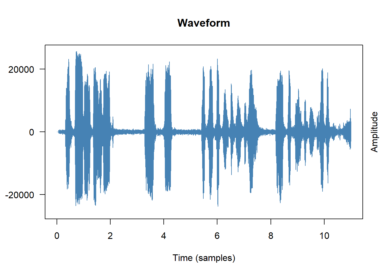
A waveform plots amplitude (air pressure displacement) against time. It shows when the recording is loud or quiet, where there are pauses, and whether the signal is clipped (amplitude maxed out):

# Base R plot method for Wave objects  
plot(wav, main = "Waveform", col = "steelblue",  
     xlab = "Time (samples)", ylab = "Amplitude")  

From the waveform you can immediately see:

• Pauses and silences — flat regions with near-zero amplitude
  
• Clipping — amplitude that hits the maximum value consistently
  
• Background noise — a non-zero baseline even during silence
  
• Approximate speech rhythm — alternating loud (vowel nuclei) and quiet (consonants) regions

Spectrogram

A spectrogram plots frequency (y-axis) against time (x-axis), with colour representing intensity. It reveals the frequency structure of speech — formants, fricatives, stop bursts — that the waveform cannot show:

# Narrow-band spectrogram (good for pitch/formants)  
seewave::spectro(wav,  
                 flim = c(0, 8),      # frequency limit in kHz  
                 main = "Spectrogram",  
                 collevels = seq(-40, 0, 1))   # dynamic range in dB  
  
# Wide-band spectrogram (good for temporal structure)  
seewave::spectro(wav,  
                 wl = 256,            # shorter window = better time resolution  
                 flim = c(0, 8),  
                 main = "Wide-band Spectrogram")  

Reading a Spectrogram

In a spectrogram of speech:

• Dark horizontal bands (especially in the lower 3 kHz) are formants — resonant frequencies of the vocal tract that define vowel quality
  
• Broadband vertical striations are voicing pulses from the vocal folds
  
• Diffuse high-frequency energy indicates fricatives (s, f, sh)
  
• Silence / gaps appear as blank regions
  
• The fundamental frequency (F0) is the lowest horizontal band and its harmonics are visible as evenly spaced bands above it
  

---

Exercises: Audio Basics

Q1. What does a sampling rate of 16,000 Hz mean?

The audio file is 16,000 bytes in size
The recording lasted 16,000 seconds
The audio contains frequencies up to 16,000 kHz
16,000 amplitude measurements are taken per second when recording the audio

---

Q2. What does a spectrogram show that a waveform does not?

The frequency content of the signal over time — which frequencies are present and how their intensity changes
The total duration of the recording
The amplitude of the signal at each moment in time
The file size and bit depth of the audio

---

Voice Activity Detection (VAD)

Section Overview

What you’ll learn: How to use the built-in Silero VAD in audio.whisper to identify speech segments and split audio on pauses — the correct way to segment long recordings

Key function: audio.whisper::vad()

Why it matters: Splitting on fixed time intervals (e.g., every 5 seconds) is almost always wrong — it cuts through words mid-utterance. VAD splits at natural pause boundaries where there is genuinely no speech.

What Is VAD?

Voice Activity Detection classifies each moment in the audio as either speech or non-speech (silence, background noise, music). In a transcription pipeline, VAD serves two purposes:

1. Pre-segmentation: Split a long recording into shorter chunks at natural pause boundaries before sending to Whisper, so that each segment is self-contained
   
2. Noise filtering: Prevent Whisper from wasting computation (and producing hallucinated output) on silent or non-speech portions

audio.whisper integrates the Silero VAD model — a lightweight, accurate voice activity detector — directly into the package. No additional installation is needed.

Running VAD

# Detect speech segments in the audio file  
vad_result <- audio.whisper::vad(  
  path                 = audio_path,  
  threshold            = 0.5,    # confidence threshold: 0–1 (higher = stricter)  
  min_speech_duration  = 250,    # minimum speech segment in ms  
  min_silence_duration = 100,    # minimum silence to split on, in ms  
  max_speech_duration  = -1,     # no maximum (set to e.g. 30000 for 30s chunks)  
  pad                  = 30,     # pad each segment by this many ms  
  overlap              = 0.1     # seconds of overlap between segments  
)  
  
# Inspect the result  
head(vad_result$data)  

  segment  from    to has_voice
1       1 0.029 0.221      TRUE
2       2 0.330 0.377      TRUE
3       3 0.400 0.435      TRUE
4       4 0.538 0.765      TRUE
5       5 0.816 1.059      TRUE

The $data element is a data frame with columns segment, from, to, and has_voice:

segment	from	to	has_voice
1	0.00	1.19	false
2	1.24	3.76	true
3	3.81	5.05	false
4	5.10	7.28	true
5	7.34	8.97	false
6	9.02	11.00	true

Extracting Speech Segments for Transcription

# Keep only the speech segments  
speech_segments <- vad_result$data |>  
  dplyr::filter(has_voice == TRUE)  
  
# These timestamps can be passed directly to Whisper's sections argument  
# Convert from seconds to milliseconds for the sections argument  
sections <- data.frame(  
  start    = as.integer(speech_segments$from * 1000),  
  duration = as.integer((speech_segments$to - speech_segments$from) * 1000)  
)  
  
cat("Found", nrow(sections), "speech segments\n")  

Found 5 speech segments

cat("Total speech duration:", sum(sections$duration) / 1000, "seconds\n")  

Total speech duration: 0.741 seconds

VAD vs. Fixed-Length Chunking

The draft of this tutorial suggested splitting audio into fixed 5-second chunks. This is almost always the wrong approach. Fixed chunking:

• Cuts through words and sentences mid-utterance
  
• Forces Whisper to transcribe fragments with no linguistic context
  
• Produces transcripts that are hard to reassemble

VAD-based splitting respects linguistic structure: it splits at silence boundaries where speakers have paused. Each segment is a complete utterance or breath group, giving Whisper maximum context and producing much cleaner output.

The only situation where fixed-length chunking is appropriate is when the audio has no natural pauses (e.g., continuous singing, non-stop machine noise) — not typical for speech data.

---

Automatic Speech Recognition with Whisper

Section Overview

What you’ll learn: How to download Whisper models, transcribe audio files, and work with the time-aligned output

Key functions: audio.whisper::whisper(), predict()

Why R, not Python: audio.whisper is an Rcpp wrapper around whisper.cpp — a highly optimised C++ implementation of Whisper. It runs entirely within R with no Python dependency.

What Is Whisper?

Whisper is OpenAI’s open-source automatic speech recognition model, released in 2022 and updated regularly since. Key properties:

• Trained on over 680,000 hours of multilingual audio from the web
  
• Supports transcription in ~100 languages and translation to English
  
• Available in five sizes — from tiny (39M parameters) to large-v3 (1.5B parameters)
  
• Robust to accents, background noise, and technical vocabulary
  
• Produces word-level timestamps when requested
  
• Released under the MIT licence — free for academic and commercial use

Whisper’s architecture is a transformer-based encoder-decoder. Audio is converted into a log-Mel spectrogram, processed by the encoder, and decoded into text tokens by the decoder. The training procedure exposes the model to extremely diverse speech conditions, giving it strong zero-shot generalisation.

Whisper Model Sizes

Model	Parameters	Download_size	RAM_required	Notes
tiny	39M	75 MB	~390 MB	Fastest, lowest accuracy
tiny.en	39M	75 MB	~390 MB	English only
base	74M	142 MB	~500 MB	Good balance for testing
base.en	74M	142 MB	~500 MB	English only
small	244M	466 MB	~1.0 GB	Recommended starting point
small.en	244M	466 MB	~1.0 GB	English only
medium	769M	~1.4 GB	~2.6 GB	Good multilingual accuracy
medium.en	769M	~1.4 GB	~2.6 GB	English only
large-v2	1.5B	~2.9 GB	~5.0 GB	High accuracy
large-v3	1.5B	~2.9 GB	~5.0 GB	Best accuracy
large-v3-turbo	809M	~1.5 GB	~3.1 GB	Fast + high accuracy (recommended)

Downloading a Model

Models are downloaded from HuggingFace and cached locally. You only need to download each model once:

# Download a model — specify the model name  
# The model file is stored in R's user data directory  
whisper_download_model("base")      # 142 MB — good for testing  
whisper_download_model("small")     # 466 MB — recommended for research  
whisper_download_model("large-v3-turbo")  # best accuracy/speed trade-off  

Basic Transcription

# Load the model  
model <- audio.whisper::whisper("base")  
  
# Transcribe the audio file  
trans <- predict(model,  
                 newdata  = audio_path,  
                 language = "en",    # specify language or "auto" for detection  
                 n_threads = 4)      # use multiple CPU threads for speed  
  
# Inspect the result  
trans  

The output of predict() is a list with three elements:

Element	Type	Contains
$data	data.frame	Segment-level transcript: columns segment, segment_offset, text, from, to
$tokens	data.frame	Token-level transcript: segment, token_id, token, token_prob (if token_timestamps = TRUE)
$timing	list	Start, end, and duration of the transcription process

# The main transcript: one row per segment  
head(trans$data)  
  
# Number of segments transcribed  
nrow(trans$data)  
  
# Plain text: concatenate all segments  
full_text <- paste(trans$data$text, collapse = " ")  
cat(full_text)  

Time-Aligned Segments

The $data data frame includes from and to columns in HH:MM:SS.mmm format — the start and end time of each segment in the audio:

# View the time-aligned transcript  
trans$data |>  
  dplyr::select(segment, from, to, text) |>  
  head(10)  

A simulated example of what this looks like:

segment	from	to	text
1	00:00:00.000	00:00:02.280	And so my fellow Americans,
2	00:00:02.340	00:00:05.710	ask not what your country can do for you,
3	00:00:05.780	00:00:09.060	ask what you can do for your country.
4	00:00:09.120	00:00:12.490	My fellow citizens of the world,
5	00:00:12.560	00:00:15.200	ask not what America will do for you,

Token-Level Timestamps

Setting token_timestamps = TRUE provides token-level alignment — each subword token gets its own time range and probability score:

trans_tokens <- predict(model,  
                        newdata           = audio_path,  
                        language          = "en",  
                        token_timestamps  = TRUE,  
                        n_threads         = 4)  
  
# Token-level output  
head(trans_tokens$tokens, 15)  

Token timestamps are useful for forced alignment — connecting specific words to precise time positions in the audio. They are less accurate than dedicated forced aligner tools (such as the Montreal Forced Aligner), but require no additional setup and are good enough for many research purposes.

Transcribing VAD-Segmented Audio

For longer recordings, the recommended workflow is to run VAD first and pass the speech segments to predict() via the sections argument:

# Run VAD  
vad_result <- audio.whisper::vad(audio_path)  
  
# Extract speech segments, convert to ms  
sections <- vad_result$data |>  
  dplyr::filter(has_voice == TRUE) |>  
  dplyr::transmute(  
    start    = as.integer(from * 1000),  
    duration = as.integer((to - from) * 1000)  
  )  
  
# Transcribe only the speech segments  
model <- audio.whisper::whisper("small")  
trans <- predict(model,  
                 newdata   = audio_path,  
                 language  = "en",  
                 sections  = sections,  
                 n_threads = 4)  
  
nrow(trans$data)  
head(trans$data[, c("segment", "from", "to", "text")])  

Using VAD Built into predict()

Alternatively, predict() accepts a vad = TRUE argument that runs Silero VAD internally before transcription — a convenient one-step approach:

model <- audio.whisper::whisper("small")  
  
trans <- predict(model,  
                 newdata   = audio_path,  
                 language  = "en",  
                 vad       = TRUE,    # run VAD automatically  
                 n_threads = 4)  
  
head(trans$data[, c("from", "to", "text")])  

---

Exercises: ASR with Whisper

Q1. Why should you use vad = TRUE or pre-segment with vad() for long recordings rather than passing the whole file directly to predict()?

VAD removes silence and non-speech before transcription, preventing Whisper from hallucinating content for silent portions and improving both speed and accuracy
VAD converts the audio to 16 kHz, which Whisper requires
Whisper cannot process audio files longer than 30 seconds without VAD
VAD is only needed when the audio contains multiple languages

---

Q2. What is the difference between trans$data and trans$tokens?

They contain identical information in different formats
$data is for English; $tokens is for other languages
$data contains one row per recognised segment with start/end timestamps; $tokens contains one row per subword token with individual probabilities (only available with token_timestamps = TRUE)
$tokens is faster to produce than $data

---

Q3. Which Whisper model is recommended as the best balance between speed and accuracy for most research use cases?

"base" — it is the only model that runs without a GPU
"large-v3-turbo" — it achieves near large-v3 accuracy at roughly half the computational cost
"tiny" — it is the fastest model and accuracy differences are minimal
"medium.en" — it is the largest English-only model

---

Translation

Section Overview

What you’ll learn: How to use Whisper’s built-in translation capability to transcribe non-English audio directly into English

Key argument: type = "translate" in predict()

One of Whisper’s most useful capabilities for linguistic research is speech-to-text translation: transcribing audio in one language directly into English text — without a separate translation step. This is particularly valuable for multilingual corpora where you want English translations of non-English speech.

# Transcribe in the original language (e.g., Dutch)  
trans_nl <- predict(model,  
                    newdata  = audio_path_dutch,  
                    language = "nl",  
                    type     = "transcribe")   # default  
  
# Translate to English  
trans_en <- predict(model,  
                    newdata  = audio_path_dutch,  
                    language = "nl",  
                    type     = "translate")    # produces English output  
  
# Compare  
cat("Dutch:   ", paste(trans_nl$data$text, collapse = " "), "\n")  
cat("English: ", paste(trans_en$data$text, collapse = " "), "\n")  

Supported Languages

To see all languages Whisper supports:

audio.whisper::whisper_languages()  

Whisper supports ~100 languages. Performance varies considerably: accuracy is highest for high-resource languages (English, Spanish, French, German, Chinese, Japanese) and lower for low-resource languages. Always evaluate accuracy on a sample of your own data before relying on Whisper for a full corpus.

---

Speaker Diarisation

Section Overview

What you’ll learn: How to identify which speaker uttered each segment of a multi-speaker recording

Key argument: diarize = TRUE in predict()

Why it matters: Without diarisation, a transcript of a conversation or interview shows only sequential text with no indication of speaker turns. Diarisation adds the “who spoke when” dimension that is essential for conversation analysis, sociolinguistics, and interview research.

What Is Speaker Diarisation?

Speaker diarisation is the process of partitioning an audio stream into segments and labelling each segment with the identity (or an anonymous label) of the speaker. It answers the question: “Who spoke when?”

Diarisation does not identify who a person is by name — it assigns arbitrary labels (SPEAKER_00, SPEAKER_01, etc.) that are consistent within a recording. Two utterances from the same physical speaker receive the same label; utterances from different speakers receive different labels.

The typical pipeline is:

Audio → VAD → Speaker Embedding Extraction → Clustering → Label Assignment  

Running Diarisation with audio.whisper

audio.whisper supports diarisation directly within predict() via the diarize = TRUE argument:

model <- audio.whisper::whisper("small")  
  
trans_diarised <- predict(model,  
                          newdata   = audio_path,  
                          language  = "en",  
                          diarize   = TRUE,    # enable speaker diarisation  
                          vad       = TRUE,    # also enable VAD  
                          n_threads = 4)  
  
# The $data column now includes a 'speaker' column  
head(trans_diarised$data[, c("segment", "from", "to", "speaker", "text")])  

segment	from	to	speaker	text
1	00:00:00.000	00:00:03.350	SPEAKER_00	Good morning, can you tell me about your research?
2	00:00:03.400	00:00:07.060	SPEAKER_01	Yes, I work on language acquisition in bilingual children.
3	00:00:07.120	00:00:10.820	SPEAKER_00	Fascinating. What age group do you focus on?
4	00:00:10.880	00:00:14.180	SPEAKER_01	Primarily three to six year olds, the critical period.
5	00:00:14.230	00:00:18.690	SPEAKER_00	And what methods do you typically use?
6	00:00:18.750	00:00:22.400	SPEAKER_01	Mainly naturalistic observation and structured elicitation tasks.

Working with Diarised Transcripts

# How many turns per speaker?  
trans_diarised$data |>  
  dplyr::count(speaker, sort = TRUE)  
  
# How much time does each speaker occupy?  
trans_diarised$data |>  
  dplyr::mutate(  
    from_sec = as.numeric(substr(from, 7, 12)),  
    to_sec   = as.numeric(substr(to,   7, 12)),  
    duration = to_sec - from_sec  
  ) |>  
  dplyr::group_by(speaker) |>  
  dplyr::summarise(  
    n_turns    = dplyr::n(),  
    total_sec  = round(sum(duration), 1),  
    mean_turn  = round(mean(duration), 2),  
    .groups    = "drop"  
  )  
  
# Extract one speaker's contribution only  
speaker_00_text <- trans_diarised$data |>  
  dplyr::filter(speaker == "SPEAKER_00") |>  
  dplyr::pull(text) |>  
  paste(collapse = " ")  

Limitations of Built-in Diarisation

audio.whisper’s built-in diarisation is convenient but limited compared to dedicated tools:

• It uses speaker embeddings derived from the Whisper encoder, not a purpose-built diarisation model
  
• Accuracy degrades with more than 3–4 speakers or significant speaker overlap
  
• It cannot handle cross-talk (simultaneous speech)

For more accurate diarisation, especially for long recordings with many speakers or overlapping speech, consider post-processing with pyannote.audio (Python) or matching Whisper’s segment timestamps against a separate diarisation tool.

---

Post-Processing Transcripts

Section Overview

What you’ll learn: How to clean, structure, save, and begin analysing transcripts produced by Whisper

Key operations: Text cleaning, timestamp parsing, saving to CSV/text formats

Whisper output typically requires some post-processing before analysis. Common steps include removing leading/trailing whitespace, standardising punctuation, parsing timestamps, and saving in corpus-friendly formats.

Cleaning the Transcript

library(stringr)  
  
transcript_clean <- trans$data |>  
  dplyr::mutate(  
    # Remove leading/trailing whitespace (Whisper adds a leading space to each segment)  
    text     = stringr::str_trim(text),  
    # Normalise multiple spaces  
    text     = stringr::str_replace_all(text, "\\s+", " "),  
    # Remove segments that are likely hallucinations (very short or only punctuation)  
    is_valid = stringr::str_detect(text, "[[:alpha:]]{3,}")  
  ) |>  
  dplyr::filter(is_valid) |>  
  dplyr::select(-is_valid)  

Parsing Timestamps

Whisper returns timestamps as HH:MM:SS.mmm strings. Convert them to numeric seconds for calculations:

parse_hms <- function(hms_string) {  
  # Convert "HH:MM:SS.mmm" to numeric seconds  
  parts <- stringr::str_split(hms_string, "[:.]")[[1]]  
  h <- as.numeric(parts[1])  
  m <- as.numeric(parts[2])  
  s <- as.numeric(parts[3])  
  ms <- as.numeric(parts[4]) / 1000  
  h * 3600 + m * 60 + s + ms  
}  
  
transcript_timed <- transcript_clean |>  
  dplyr::mutate(  
    from_sec  = sapply(from, parse_hms),  
    to_sec    = sapply(to,   parse_hms),  
    duration  = to_sec - from_sec  
  )  
  
# Summary statistics  
cat("Total segments:  ", nrow(transcript_timed), "\n")  
cat("Total duration:  ", round(sum(transcript_timed$duration), 1), "seconds\n")  
cat("Mean seg. length:", round(mean(transcript_timed$duration), 2), "seconds\n")  

Saving Transcripts

# Save as CSV (best for further analysis in R)  
write.csv(transcript_timed,  
          file      = here::here("outputs", "transcript.csv"),  
          row.names = FALSE)  
  
# Save as plain text (one segment per line with timestamps)  
transcript_txt <- transcript_timed |>  
  dplyr::mutate(  
    line = paste0("[", from, " --> ", to, "] ", text)  
  ) |>  
  dplyr::pull(line)  
  
writeLines(transcript_txt, here::here("outputs", "transcript.txt"))  
  
# Save in SubRip (SRT) subtitle format — useful for video annotation  
srt_lines <- character(nrow(transcript_timed) * 4)  
for (i in seq_len(nrow(transcript_timed))) {  
  idx <- (i - 1) * 4  
  srt_lines[idx + 1] <- as.character(i)  
  srt_lines[idx + 2] <- paste(  
    gsub("\\.", ",", transcript_timed$from[i]),  
    "-->",  
    gsub("\\.", ",", transcript_timed$to[i])  
  )  
  srt_lines[idx + 3] <- transcript_timed$text[i]  
  srt_lines[idx + 4] <- ""  
}  
writeLines(srt_lines, here::here("outputs", "transcript.srt"))  

---

Extracting Acoustic Features

Section Overview

What you’ll learn: How to extract vowel formants (F1, F2) from audio and visualise the vowel space

Key functions: seewave::formant(), ggplot2

Why it matters: Formants are the primary acoustic correlates of vowel quality — the basis of sociophonetic research, vowel change studies, and second-language acquisition research

What Are Formants?

Formants are resonant frequencies of the vocal tract. Each vowel is characterised by a distinctive pattern of formant frequencies:

• F1 (first formant) correlates primarily with tongue height — low vowels have high F1, high vowels have low F1
  
• F2 (second formant) correlates primarily with tongue backness — front vowels have high F2, back vowels have low F2
  
• F3 (third formant) is associated with lip rounding and retroflexion

Plotting F1 against F2 (with axes reversed to match the traditional vowel trapezoid) shows the vowel space of a speaker or variety.

Extracting Formants

# Extract formants using seewave  
# wl: window length (samples); higher = better frequency resolution  
formants_raw <- seewave::formant(wav,  
                                 fmax  = 5500,   # maximum frequency in Hz  
                                 wl    = 512,  
                                 plot  = FALSE)  
  
# Convert to data frame  
formant_df <- as.data.frame(formants_raw)  
names(formant_df)[1:3] <- c("time", "F1", "F2")  
  
head(formant_df)  

Formant Extraction Quality

Automatic formant extraction is sensitive to:

• Voiced vs. unvoiced segments: formants are only meaningful during voiced speech. Always filter to voiced segments (where pitch is detected) before analysis.
  
• Speaker sex/age: typical F1/F2 ranges differ by speaker characteristics. Filter out implausible values (e.g., F1 > 1000 Hz or F2 < 500 Hz often indicate extraction errors).
  
• Window size: a longer analysis window gives better frequency resolution but worse time resolution. The default wl = 512 is a reasonable starting point.

For high-quality formant extraction in sociophonetics, dedicated tools like Praat (with an R interface via the rPraat or PraatR packages) are generally preferred.

Filtering and Plotting the Vowel Space

# Filter to plausible formant values (crude voiced speech filter)  
formant_filtered <- formant_df |>  
  dplyr::filter(  
    F1 > 200, F1 < 1000,   # typical F1 range for adult speakers  
    F2 > 500, F2 < 3500    # typical F2 range for adult speakers  
  ) |>  
  dplyr::filter(!is.na(F1), !is.na(F2))  
  
# Vowel space plot following phonetic convention (axes reversed)  
ggplot(formant_filtered, aes(x = F2, y = F1)) +  
  geom_point(alpha = 0.3, size = 1.2, colour = "steelblue") +  
  geom_density_2d(colour = "tomato", linewidth = 0.5) +  
  scale_x_reverse(name = "F2 (Hz)") +  
  scale_y_reverse(name = "F1 (Hz)") +  
  labs(  
    title    = "Vowel Space (F1 – F2 Plot)",  
    subtitle = "Each point = one analysis frame; contours show density"  
  ) +  
  theme_bw() +  
  theme(panel.grid.minor = element_blank())  

Connecting Acoustics to the Transcript

The most powerful analyses combine the time-aligned transcript with the acoustic measurements — extracting formants only during specific words or vowels:

# Suppose we want formants during a specific word in the transcript  
target_segment <- transcript_timed |>  
  dplyr::filter(stringr::str_detect(text, regex("\\bask\\b",  
                                                 ignore_case = TRUE))) |>  
  dplyr::slice(1)  
  
# Extract formants for the time window of that word  
# (sampling_rate was defined when loading the audio)  
start_sample <- round(target_segment$from_sec * wav@samp.rate)  
end_sample   <- round(target_segment$to_sec   * wav@samp.rate)  
  
wav_segment <- tuneR::extractWave(wav,  
                                  from   = start_sample,  
                                  to     = end_sample,  
                                  xunit  = "samples")  
  
formants_word <- seewave::formant(wav_segment, fmax = 5500, plot = FALSE)  

This kind of targeted extraction — formants during specific words, identified via their Whisper-generated timestamps — is the core workflow for corpus phonetics and sociophonetics research.

---

Exercises: Acoustics and Post-Processing

Q1. Why are the axes reversed in an F1–F2 vowel space plot?

Because ggplot2 requires reversed axes for frequency data
To match the traditional vowel trapezoid: high F1 (low vowels) appears at the bottom, low F1 (high vowels) at the top; high F2 (front vowels) on the left, low F2 (back vowels) on the right
Because F1 and F2 values are always negative numbers
To make the plot look more like a spectrogram

---

Q2. What is the purpose of filtering formant values to F1 > 200 & F1 < 1000 before plotting?

Because Whisper only transcribes speech in this frequency range
Because ggplot2 cannot plot values outside this range
To reduce the file size of the plot
To exclude likely extraction errors — formants are only meaningful during voiced vowels, and implausible values typically reflect unvoiced segments, consonants, or algorithm failures

---

Summary

This tutorial has covered the complete speech processing pipeline in R, from raw audio to linguistic analysis:

Audio handling (tuneR): loading WAV files, inspecting sampling rate and duration, generating waveforms and spectrograms.

Voice Activity Detection (audio.whisper::vad()): splitting recordings on natural pause boundaries using the Silero VAD model — the correct alternative to fixed-length chunking.

Automatic Speech Recognition (audio.whisper): downloading Whisper models, transcribing audio in any of ~100 languages, obtaining time-aligned segment and token output, using VAD pre-filtering to reduce hallucination.

Translation (type = "translate"): converting non-English speech directly to English text.

Speaker diarisation (diarize = TRUE): labelling which speaker produced each segment, enabling conversation and interview analysis.

Post-processing: cleaning Whisper output, parsing timestamps to seconds, saving in CSV, TXT, and SRT formats.

Acoustic feature extraction (seewave::formant()): extracting vowel formants and visualising the vowel space, including targeted extraction for specific words using transcript timestamps.

The unifying theme is the pipeline: each step produces structured data — timestamps, text, speaker labels, formant measurements — that can be combined with dplyr for linguistically meaningful analyses.

---

Citation & Session Info

Citation

Martin Schweinberger. 2026. Speech Processing in R: Transcription and Analysis with Whisper. The Language Technology and Data Analysis Laboratory (LADAL), The University of Queensland, Australia. url: https://ladal.edu.au/tutorials/speechprocessing/speechprocessing.html (Version 2026.03.28), doi: .

@manual{martinschweinberger2026speech,
  author       = {Martin Schweinberger},
  title        = {Speech Processing in R: Transcription and Analysis with Whisper},
  year         = {2026},
  note         = {https://ladal.edu.au/tutorials/speechprocessing/speechprocessing.html},
  organization = {The Language Technology and Data Analysis Laboratory (LADAL), The University of Queensland, Australia},
  edition      = {2026.03.28}
  doi      = {}
}

sessionInfo()  

R version 4.4.2 (2024-10-31 ucrt)
Platform: x86_64-w64-mingw32/x64
Running under: Windows 11 x64 (build 26200)

Matrix products: default


locale:
[1] LC_COLLATE=English_United States.utf8 
[2] LC_CTYPE=English_United States.utf8   
[3] LC_MONETARY=English_United States.utf8
[4] LC_NUMERIC=C                          
[5] LC_TIME=English_United States.utf8    

time zone: Australia/Brisbane
tzcode source: internal

attached base packages:
[1] stats     graphics  grDevices datasets  utils     methods   base     

other attached packages:
[1] here_1.0.2          audio.whisper_0.5.0 flextable_0.9.11   
[4] checkdown_0.0.13    ggplot2_4.0.2       dplyr_1.2.0        
[7] reticulate_1.44.1   seewave_2.2.4       tuneR_1.4.7        

loaded via a namespace (and not attached):
 [1] generics_0.1.3          tidyr_1.3.2             fontLiberation_0.1.0   
 [4] renv_1.1.7              xml2_1.3.6              lattice_0.22-6         
 [7] digest_0.6.39           magrittr_2.0.3          evaluate_1.0.3         
[10] grid_4.4.2              RColorBrewer_1.1-3      fastmap_1.2.0          
[13] rprojroot_2.1.1         jsonlite_1.9.0          Matrix_1.7-2           
[16] zip_2.3.2               purrr_1.0.4             scales_1.4.0           
[19] fontBitstreamVera_0.1.1 codetools_0.2-20        textshaping_1.0.0      
[22] cli_3.6.4               rlang_1.1.7             fontquiver_0.2.1       
[25] litedown_0.9            commonmark_2.0.0        withr_3.0.2            
[28] yaml_2.3.10             gdtools_0.5.0           tools_4.4.2            
[31] officer_0.7.3           uuid_1.2-1              vctrs_0.7.1            
[34] R6_2.6.1                png_0.1-8               lifecycle_1.0.5        
[37] htmlwidgets_1.6.4       MASS_7.3-61             ragg_1.3.3             
[40] pkgconfig_2.0.3         pillar_1.10.1           gtable_0.3.6           
[43] glue_1.8.0              data.table_1.17.0       Rcpp_1.1.1             
[46] systemfonts_1.3.1       xfun_0.56               tibble_3.2.1           
[49] tidyselect_1.2.1        rstudioapi_0.17.1       knitr_1.51             
[52] farver_2.1.2            patchwork_1.3.0         htmltools_0.5.9        
[55] rmarkdown_2.30          signal_1.8-1            compiler_4.4.2         
[58] S7_0.2.1                askpass_1.2.1           markdown_2.0           
[61] openssl_2.3.2          

AI Transparency Statement

This tutorial was re-developed with the assistance of Claude (claude.ai), a large language model created by Anthropic. Claude was used to help revise the tutorial text, structure the instructional content, generate the R code examples, and write the checkdown quiz questions and feedback strings. All content was reviewed, edited, and approved by the author (Martin Schweinberger), who takes full responsibility for the accuracy and pedagogical appropriateness of the material. The use of AI assistance is disclosed here in the interest of transparency and in accordance with emerging best practices for AI-assisted academic content creation.

Back to top

Back to HOME

---

References