This tutorial provides a practical overview of core text analysis methods in R, covering concordancing, word frequency analysis, collocations, keywords, text classification, part-of-speech tagging, named entity recognition, and dependency parsing. It is aimed at researchers in corpus linguistics and digital humanities who want a hands-on introduction to the main computational text analysis methods available in R.
Author
Martin Schweinberger
Published
2026
Great Court, The University of Queensland
Introduction
This is Part 2 of the LADAL Introduction to Text Analysis tutorial series. Where Part 1 focused on concepts and theoretical foundations, this tutorial focuses on practical implementation: how to apply selected text analysis methods in R using real corpus data. Each section introduces a method, explains the key decisions involved, demonstrates the code, and provides exercises to consolidate understanding.
The methods covered — concordancing, word frequency analysis, collocation analysis, and keyword analysis — represent the core quantitative techniques of corpus-based text analysis. They are foundational: most more advanced analyses (topic modelling, stylometry, sentiment analysis) build upon or assume familiarity with these basic tools.
Prerequisite Tutorials
Please complete these before working through this tutorial:
Quick Reference — essential functions and workflow summary
Citation
Martin Schweinberger. 2026. Introduction to Text Analysis: Practical Implementation in R. The Language Technology and Data Analysis Laboratory (LADAL), The University of Queensland, Australia. url: https://ladal.edu.au/tutorials/textanalysis/textanalysis.html (Version 3.1.1). doi: 10.5281/zenodo.19332976.
Setup and Data
Section Overview
What you’ll learn: How to install and load the required packages, and how the tutorial data is structured
Installing Packages
Code
# Core text analysis framework
install.packages("quanteda")
install.packages("quanteda.textplots")
install.packages("quanteda.textstats")

# Data manipulation and visualisation
install.packages("dplyr")
install.packages("tidyr")
install.packages("stringr")
install.packages("ggplot2")

# Text utilities
install.packages("tidytext")
install.packages("tokenizers")
install.packages("flextable")
install.packages("here")
install.packages("checkdown")
Loading Packages
Code
library(quanteda)               # core text analysis framework
library(quanteda.textplots)     # visualisation (word clouds, networks)
library(quanteda.textstats)     # statistical measures
library(dplyr)                  # data wrangling
library(tidyr)                  # data reshaping
library(stringr)                # string processing
library(ggplot2)                # plotting
library(tidytext)               # tidy text mining
library(tokenizers)             # sentence tokenisation
library(flextable)              # formatted tables
library(here)                   # portable file paths
library(checkdown)              # interactive exercises
library(quanteda.textstats)     # for frequency analysis
Loading All Packages at the Top
Always load all required packages in a single code chunk at the top of your script. This makes dependencies immediately visible, ensures reproducibility (anyone running the script knows exactly what they need), and makes troubleshooting easier when a package is missing or out of date.
Tutorial Data
This tutorial uses Lewis Carroll’s Alice’s Adventures in Wonderland (1865), sourced from Project Gutenberg. The text is in the public domain and provides a convenient single-author literary corpus with recognisable content.
Code
# Load Alice's Adventures in Wonderland from Project Gutenberg # Using the gutenbergr package or pre-saved data # For this tutorial we load a pre-saved plain text version alice_path <- here::here("tutorials", "textanalysis", "data", "alice.rda") # Load the data (a character vector, one element per line) if (file.exists(alice_path)) { alice_raw <-readRDS(alice_path) } else { # If file not present, download directly if (!requireNamespace("gutenbergr", quietly =TRUE)) { install.packages("gutenbergr") } alice_raw <- gutenbergr::gutenberg_download(11)$text } # Quick inspection length(alice_raw)
[1] 2479
Code
head(alice_raw, 8)
[1] "Alice’s Adventures in Wonderland"
[2] "by Lewis Carroll"
[3] "CHAPTER I."
[4] "Down the Rabbit-Hole"
[5] "Alice was beginning to get very tired of sitting by her sister on the"
[6] "bank, and of having nothing to do: once or twice she had peeped into"
[7] "the book her sister was reading, but it had no pictures or"
[8] "conversations in it, “and what is the use of a book,” thought Alice"
Preparing the Text: Splitting into Chapters
For most analyses it is useful to work with the text segmented into meaningful units. We split Alice into chapters, which will serve as our “documents” in document-level analyses:
Code
# Combine all lines, mark chapter boundaries, split into chapters alice_chapters <- alice_raw |># Collapse to single string paste0(collapse =" ") |># Insert a unique marker before each chapter heading # The regex matches: "CHAPTER" + roman numerals (1-7 chars) + optional period stringr::str_replace_all("(CHAPTER [XVI]{1,7}\\.{0,1}) ", "|||\\1 ") |># Lowercase the whole text tolower() |># Split on the chapter boundary marker stringr::str_split("\\|\\|\\|") |>unlist() |># Remove any empty strings (\(x) x[nzchar(stringr::str_trim(x))])() # How many segments? cat("Number of segments:", length(alice_chapters), "\n")
Chapter 2 begins: chapter i. down the rabbit-hole alice was beginning to get v ...
Regex Explained: (CHAPTER [XVI]{1,7}\\.{0,1})
CHAPTER — matches the literal word “CHAPTER”
[XVI]{1,7} — matches 1 to 7 Roman numeral characters (I, V, X, L)
\\.{0,1} — matches an optional period (the \\. escapes the dot; {0,1} makes it optional)
The whole group is wrapped in (...) for capture. We insert ||| before each match to create a unique split point. The {0,1} is equivalent to ? — using the explicit form makes the intent clearer.
The quanteda Workflow
The quanteda package provides a consistent workflow for corpus-based text analysis built around three core objects:
Object
Created by
Contains
Used for
corpus
corpus()
Document collection with metadata
Storage, metadata management, subsetting
tokens
tokens()
Tokenised text — a list of character vectors
Concordancing, collocations, n-grams
dfm
dfm()
Document-Feature Matrix: documents × word frequencies
Frequency analysis, keywords, topic modelling, classification
cat("DFM: ", nfeat(alice_dfm), "unique features (after stopword removal)\n")
DFM: 2753 unique features (after stopword removal)
Concordancing
Section Overview
What you’ll learn: How to extract KWIC (Key Word In Context) displays using quanteda::kwic(), search with regular expressions, and search for multi-word phrases
Key function:quanteda::kwic()
When to use it: At the start of any analysis involving a specific word or phrase; to inspect how terms are used; to extract authentic examples; to identify patterns that quantitative measures cannot reveal
Concordancing is the foundation of corpus-based text analysis. Before drawing quantitative conclusions about how a word behaves, it is essential to look at actual examples and understand the range of contexts in which the word appears. The kwic() function in quanteda produces KWIC displays directly:
Simple Word Search
Code
# Concordance for "alice" — 5-word window on each side kwic_alice <- quanteda::kwic( x = alice_tokens, pattern ="alice", window =5) |>as.data.frame() |> dplyr::select(docname, pre, keyword, post) # How many occurrences? cat("Occurrences of 'alice':", nrow(kwic_alice), "\n")
Occurrences of 'alice': 386
docname
pre
keyword
post
text2
i . down the rabbit-hole
alice
was beginning to get very
text2
a book , ” thought
alice
“ without pictures or conversations
text2
in that ; nor did
alice
think it so _very_ much
text2
and then hurried on ,
alice
started to her feet ,
text2
in another moment down went
alice
after it , never once
text2
down , so suddenly that
alice
had not a moment to
text2
“ well ! ” thought
alice
to herself , “ after
text2
for , you see ,
alice
had learnt several things of
The docname column shows which chapter (document) the occurrence is from. pre is the left context, keyword is the search term, and post is the right context.
Pattern Matching with Regular Expressions
Code
# Find all word forms beginning with "walk" kwic_walk <- quanteda::kwic( x = alice_tokens, pattern ="walk.*", window =5, valuetype ="regex"# enable regular expression matching ) |>as.data.frame() |> dplyr::select(docname, pre, keyword, post) cat("Forms of 'walk':", nrow(kwic_walk), "\n")
Forms of 'walk': 20
Code
# What distinct forms were found?
unique(kwic_walk$keyword)
[1] "walk" "walking" "walked"
docname
pre
keyword
post
text2
out among the people that
walk
with their heads downward !
text2
to dream that she was
walking
hand in hand with dinah
text2
trying every door , she
walked
sadly down the middle ,
text3
“ or perhaps they won’t
walk
the way i want to
text4
mouse , getting up and
walking
away . “ you insult
text4
its head impatiently , and
walked
a little quicker . “
text5
and get ready for your
walk
! ’ ‘ coming in
text7
, “ if you only
walk
long enough . ” alice
Three valuetype Options in kwic()
"glob" (default): simple wildcards — * matches any sequence, ? matches any single character. E.g., "walk*" matches walk, walks, walked
"regex": full regular expression syntax — "walk.*" matches the same
"fixed": exact string match — "walk" matches only walk, not walks
For corpus searches, "regex" is the most powerful but also requires care with escaping special characters.
Phrase Search
Code
# Search for the multi-word phrase "poor alice" kwic_pooralice <- quanteda::kwic( x = alice_tokens, pattern = quanteda::phrase("poor alice"), # phrase() enables multi-word search window =6) |>as.data.frame() |> dplyr::select(docname, pre, keyword, post) cat("Occurrences of 'poor alice':", nrow(kwic_pooralice), "\n")
Occurrences of 'poor alice': 11
docname
pre
keyword
post
text2
would go through , ” thought
poor alice
, “ it would be of
text2
once ; but , alas for
poor alice
! when she got to the
text2
no use now , ” thought
poor alice
, “ to pretend to be
text3
off to the garden door .
poor alice
! it was as much as
text3
the right words , ” said
poor alice
, and her eyes filled with
text4
didn’t mean it ! ” pleaded
poor alice
. “ but you’re so easily
text4
any more ! ” and here
poor alice
began to cry again , for
text5
pleasanter at home , ” thought
poor alice
, “ when one wasn’t always
text6
used to it ! ” pleaded
poor alice
in a piteous tone . and
text8
. ” this answer so confused
poor alice
, that she let the dormouse
text10
both sat silent and looked at
poor alice
, who felt ready to sink
When to Use phrase() vs. a Plain Pattern
Without phrase(), a pattern like "poor alice" would be interpreted as two separate patterns. phrase() tells quanteda to look for the words adjacent to each other as a sequence. Use phrase() for:
Multi-word expressions and idioms (by and large, make a decision)
Named entities (Mad Hatter, White Rabbit)
Fixed collocations where word order matters
Sorting Concordances for Pattern Analysis
Sorting KWIC output by the left or right context makes patterns more visible:
Code
# Sort by one word to the right of the keyword (R1) # This groups concordances by what immediately follows "said" kwic_said <- quanteda::kwic( x = alice_tokens, pattern ="said", window =4) |>as.data.frame() |> dplyr::select(docname, pre, keyword, post) |># Extract the first word of the right context dplyr::mutate(R1 = stringr::word(post, 1)) |># Sort by R1 to see what typically follows "said" dplyr::arrange(R1) # Most common words following "said" kwic_said |> dplyr::count(R1, sort =TRUE) |>head(10)
        R1   n
1      the 207
2    alice 115
3       to  39
4        ,  28
5       in   7
6  nothing   6
7     this   6
8        “   5
9        .   4
10       :   3
R1
n
the
207
alice
115
to
39
,
28
in
7
nothing
6
this
6
“
5
.
4
:
3
Sorting reveals a pattern immediately: “said” is most often followed by the character names (alice, the) — the classic dialogue attribution pattern “…” said Alice.
Exercises: Concordancing
Q1. What does valuetype = "regex" do in kwic(), and why would you use it instead of the default "glob"?
Q2. You want to find all occurrences of run, runs, ran, and running in a corpus. Which pattern and valuetype combination would work correctly?
Word Frequency Analysis
Section Overview
What you’ll learn: How to build word frequency lists, handle stopwords, visualise frequency distributions, and track word frequency across document sections
When to use it: As one of the first steps in any corpus analysis; for vocabulary profiling; for identifying dominant themes; for comparing texts
Word frequency analysis counts how often each word occurs in a text or corpus. Despite its simplicity, it is one of the most informative first steps in text analysis — the vocabulary profile of a text reveals its themes, register, and style.
Building a Frequency List
Code
# Tokenise Alice, remove punctuationalice_tokens_clean <- quanteda::tokens( quanteda::corpus(paste(alice_raw, collapse =" ")),remove_punct =TRUE,remove_symbols =TRUE,remove_numbers =TRUE)# Create a DFM (no stopword removal yet)alice_dfm_all <- quanteda::dfm(alice_tokens_clean)# Extract frequency table using quanteda.textstatsfreq_all <- quanteda.textstats::textstat_frequency(alice_dfm_all) |>as.data.frame() |> dplyr::select(feature, frequency, rank)cat("Total tokens:", sum(freq_all$frequency), "\n")
The top of the frequency list is dominated by function words (the, and, to, a, of, it, she, was…) — grammatically necessary but semantically light. This is typical of English text and reflects Zipf’s Law: a small number of very frequent words account for a disproportionate share of all tokens.
Removing Stopwords
Stopwords are high-frequency function words that are removed before frequency analysis when the goal is to identify content-bearing vocabulary. The appropriate stopword list depends on the language and the research question:
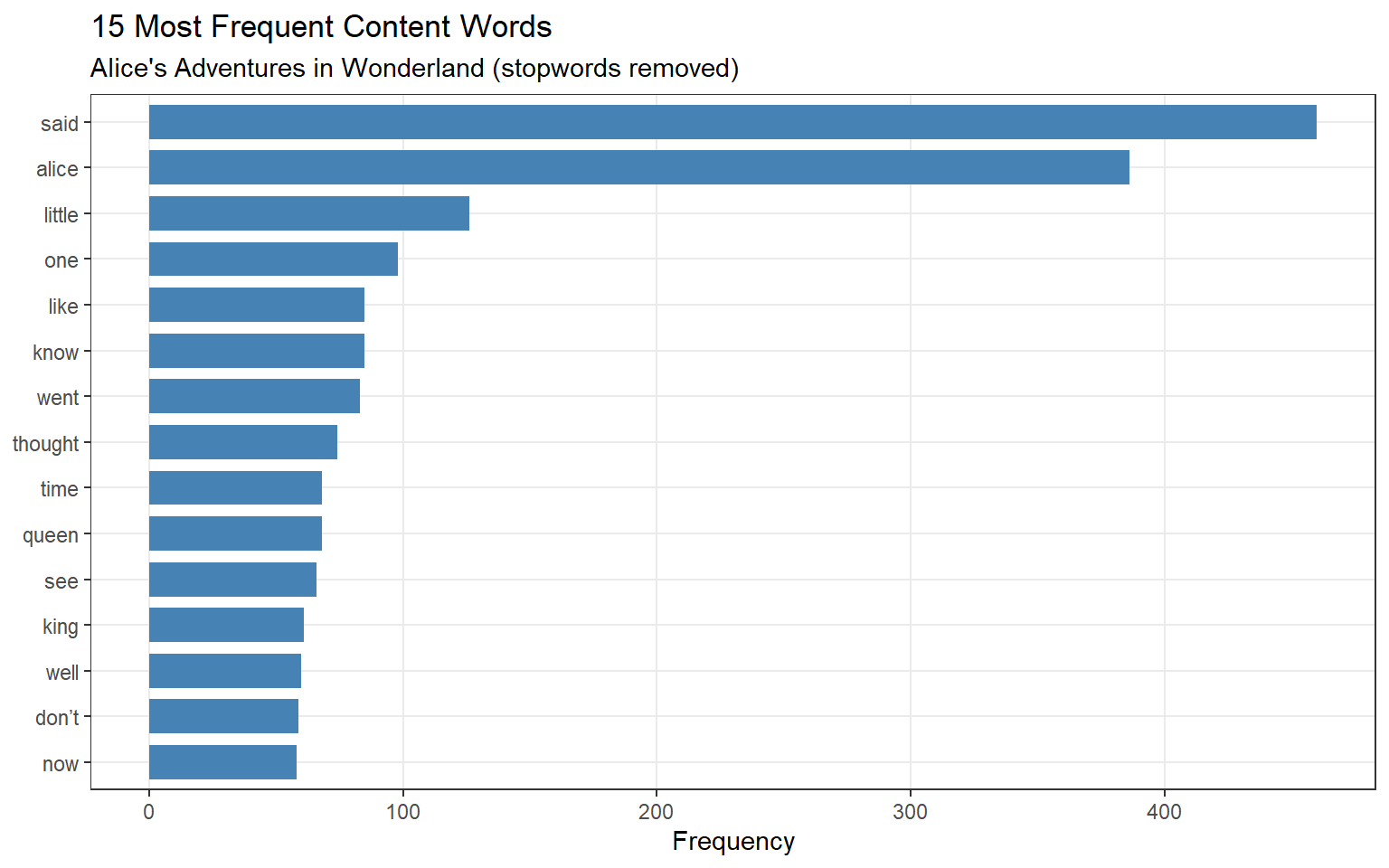
Now the list shows content words that reflect the novel’s themes: alice, said, queen, time, little, thought, king. The character alice is the most frequent content word — unsurprisingly, since the novel is named after her.
Should You Always Remove Stopwords?
Stopword removal is appropriate when analysing content (what the text is about). It is not appropriate when:
Analysing style (function word frequencies are strong style markers used in authorship attribution)
Studying discourse (function words like but, although, however carry logical structure)
Building language models (function words are necessary for grammar)
Performing concordancing (you usually want to see full context)
Always ask: does removing these words serve my research question?
Visualising Frequency
Bar Plot
Code
freq_nostop |>head(15) |>ggplot(aes(x =reorder(feature, frequency), y = frequency)) +geom_col(fill ="steelblue", width =0.75) +coord_flip() +labs( title ="15 Most Frequent Content Words", subtitle ="Alice's Adventures in Wonderland (stopwords removed)", x =NULL, y ="Frequency" ) +theme_bw() +theme(panel.grid.minor =element_blank())
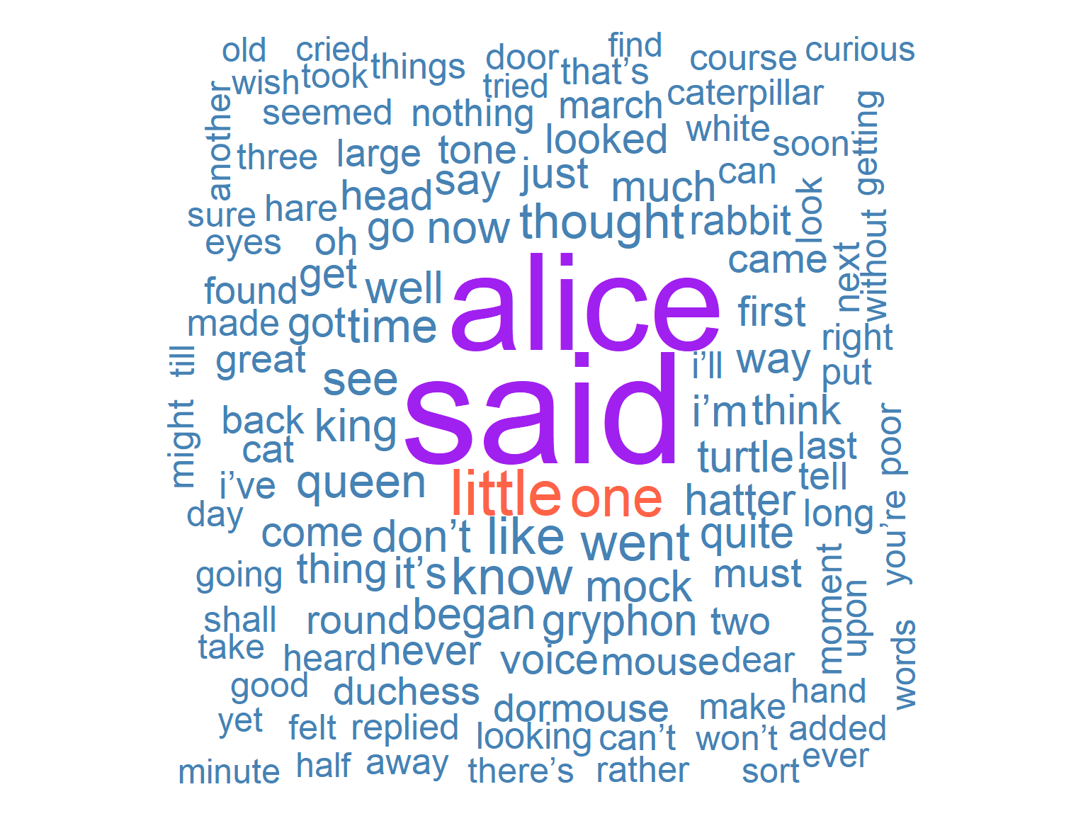
Word clouds are visually appealing and useful for exploratory work or communicating with non-specialist audiences. However, they have serious limitations as analytical tools:
It is difficult to compare sizes precisely — the visual ranking is approximate
Layout is partly random — words in the centre are not more important
They convey no information about distribution across documents
They can create misleading impressions about relative frequency
For rigorous analysis, always use bar plots or tables rather than word clouds.
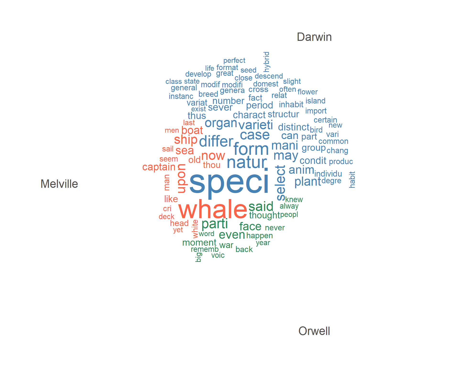
Comparison Across Authors
One of the most powerful uses of frequency analysis is comparing vocabulary across different texts or authors:
# Comparison word cloud — shows distinctive vocabulary per text # Create DFM for comparisoncomp_dfm <- comp_corpus |> quanteda::tokens(remove_punct =TRUE,remove_numbers =TRUE ) |> quanteda::tokens_tolower() |> quanteda::tokens_remove(quanteda::stopwords("english")) |> quanteda::tokens_wordstem() |> quanteda::dfm() |> quanteda::dfm_trim(min_docfreq =2)# Only plot if features remainquanteda.textplots::textplot_wordcloud( comp_dfm,comparison =TRUE,max_words =100,color =c("steelblue", "tomato", "seagreen") )
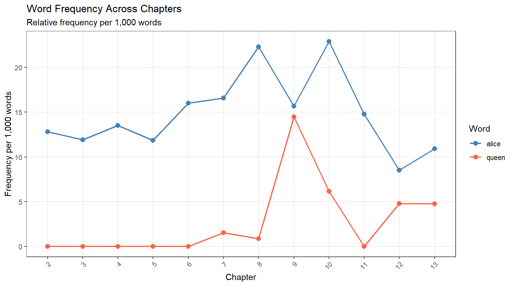
Dispersion: Frequency Across Document Sections
Tracking how word frequency changes across sections reveals narrative or structural patterns:
Code
# Count words and target word occurrences per chapter dispersion_tb <-data.frame( chapter =seq_along(alice_chapters), n_words = stringr::str_count(alice_chapters, "\\S+"), n_alice = stringr::str_count(alice_chapters, "\\balice\\b"), n_queen = stringr::str_count(alice_chapters, "\\bqueen\\b") ) |> dplyr::mutate( # Relative frequency per 1,000 words alice_per1k =round(n_alice / n_words *1000, 2), queen_per1k =round(n_queen / n_words *1000, 2), chapter_f =factor(chapter, levels = chapter) ) |> dplyr::filter(n_words >50) # exclude very short intro segments # Reshape for plotting dispersion_long <- dispersion_tb |> tidyr::pivot_longer( cols =c(alice_per1k, queen_per1k), names_to ="word", values_to ="freq_per1k" ) |> dplyr::mutate( word = dplyr::recode(word, "alice_per1k"="alice", "queen_per1k"="queen") ) ggplot(dispersion_long, aes(x = chapter_f, y = freq_per1k, colour = word, group = word)) +geom_line(linewidth =0.8) +geom_point(size =2.5) +scale_colour_manual(values =c("alice"="steelblue", "queen"="tomato")) +labs( title ="Word Frequency Across Chapters", subtitle ="Relative frequency per 1,000 words", x ="Chapter", y ="Frequency per 1,000 words", colour ="Word" ) +theme_bw() +theme(panel.grid.minor =element_blank(), axis.text.x =element_text(angle =45, hjust =1))
This dispersion plot reveals narrative structure: alice is consistently mentioned throughout, while queen appears mainly from mid-text onwards (reflecting the plot — the Queen of Hearts is introduced later in the story).
Exercises: Frequency Analysis
Q1. You build a frequency list from a news corpus and find that the is the most frequent word (frequency: 84,231). A colleague says this is important evidence that the corpus is primarily about the economy. What is wrong with this reasoning?
Q2. What does a dispersion plot show that a simple total frequency count does not?
Collocation Analysis
Section Overview
What you’ll learn: How to extract and quantify collocations — words that co-occur more than expected by chance — using co-occurrence matrices and association measures
Key concepts: Contingency table, Mutual Information (MI), phi (φ), Delta P (ΔP)
When to use it: When studying phraseological patterns, lexical associations, semantic prosody, or the characteristic usage of a target word
Collocations reveal the hidden patterning of language: every word has characteristic co-occurrence partners, and these partnerships are stable, culturally embedded, and often non-compositional. Strong coffee is a collocation; powerful coffee is not — even though strong and powerful are near-synonyms. Detecting collocations computationally requires statistical comparison: is this word pair’s co-occurrence frequency higher than we would expect if the two words were distributed independently?
The Contingency Table Approach
Collocation strength is measured using a 2×2 contingency table that cross-tabulates the presence and absence of two words:
w₂ present
w₂ absent
w₁ present
O₁₁
O₁₂
= R₁
w₁ absent
O₂₁
O₂₂
= R₂
= C₁
= C₂
= N
Where O₁₁ = both words co-occur in the same context window, O₁₂ = w₁ appears but not w₂, O₂₁ = w₂ appears but not w₁, and O₂₂ = neither appears. N is the total number of co-occurrence opportunities (contexts).
From observed (O) counts we compute expected (E) counts under the assumption of independence: E₁₁ = R₁ × C₁ / N. Association measures compare O₁₁ to E₁₁: if O₁₁ >> E₁₁, the words co-occur more than chance and are likely collocates.
Preparing Sentence-Level Data
For collocation analysis, we compute co-occurrences within sentences (rather than the whole text), so that bank and interest are counted as co-occurring only when they appear in the same sentence:
Code
# Tokenise Alice into sentences, then clean alice_sentences <-paste(alice_raw, collapse =" ") |> tokenizers::tokenize_sentences() |>unlist() |> stringr::str_replace_all("[^[:alnum:] ]", " ") |> stringr::str_squish() |>tolower() |> (\(x) x[nchar(x) >5])() # remove very short fragments cat("Number of sentences:", length(alice_sentences), "\n")
Number of sentences: 1585
Building the Co-occurrence Matrix
Code
# Create a Feature Co-occurrence Matrix (FCM) # FCM counts how often any two words appear in the same sentence coll_fcm <- alice_sentences |> quanteda::tokens() |> quanteda::dfm() |> quanteda::fcm(tri =FALSE) # tri=FALSE: count both (w1,w2) and (w2,w1) # Convert to long-format data frame coll_basic <- tidytext::tidy(coll_fcm) |> dplyr::rename(w1 = term, w2 = document, O11 = count) cat("Unique word pairs:", nrow(coll_basic), "\n")
Unique word pairs: 274011
Computing Association Measures
Code
# Compute the full contingency table and association measures coll_stats <- coll_basic |> dplyr::mutate(N =sum(O11)) |> dplyr::group_by(w1) |> dplyr::mutate(R1 =sum(O11), O12 = R1 - O11, R2 = N - R1) |> dplyr::ungroup() |> dplyr::group_by(w2) |> dplyr::mutate(C1 =sum(O11), O21 = C1 - O11, C2 = N - C1, O22 = R2 - O21) |> dplyr::ungroup() |> dplyr::mutate( # Expected co-occurrence under independence E11 = R1 * C1 / N, E12 = R1 * C2 / N, E21 = R2 * C1 / N, E22 = R2 * C2 / N, # Association measures MI =log2(O11 / E11), # Mutual Information X2 = (O11 - E11)^2/E11 + (O12 - E12)^2/E12 + (O21 - E21)^2/E21 + (O22 - E22)^2/E22, # Chi-square phi =sqrt(X2 / N), # Effect size (phi) DeltaP = (O11/(O11 + O12)) - (O21/(O21 + O22)) # Directional measure )
Collocates of a Target Word
Code
# Find collocates of "alice" alice_colls <- coll_stats |> dplyr::filter( w1 =="alice", (O11 + O21) >=10, # w2 must occur at least 10 times in the corpus O11 >=5# must co-occur at least 5 times with alice ) |># Bonferroni-corrected significance filter via chi-square dplyr::filter(X2 >qchisq(0.99, 1)) |># Keep only attraction collocates (observed > expected) dplyr::filter(O11 > E11) |> dplyr::arrange(dplyr::desc(phi))
w1
w2
O11
E11
phi
MI
DeltaP
alice
said
179
87.539
0.010
1.032
0.010
alice
thought
60
22.086
0.009
1.442
0.004
alice
very
86
53.588
0.005
0.682
0.003
alice
turning
7
1.622
0.005
2.110
0.001
alice
replied
14
5.127
0.004
1.449
0.001
alice
afraid
10
3.200
0.004
1.644
0.001
alice
asked
5
1.176
0.004
2.089
0.000
alice
to
334
276.236
0.004
0.274
0.006
alice
i
163
128.033
0.003
0.348
0.004
alice
politely
5
1.404
0.003
1.832
0.000
alice
cried
10
3.962
0.003
1.336
0.001
alice
much
32
19.441
0.003
0.719
0.001
Interpreting the Association Measures
O11: Raw co-occurrence count — how many times the pair actually appeared together
E11: Expected count under independence — how often they would co-occur if word choice were random
MI (Mutual Information): Measures how much information one word provides about the other. MI > 0 means positive association; MI >> 0 means strong association. Biased toward rare words.
DeltaP: Directional measure — how much does seeing w1 increase the probability of seeing w2? A positive value means w2 is more likely given w1.
For a corpus linguistics audience, phi and Delta P are generally the most interpretable measures. MI is commonly used in computational linguistics but can inflate the importance of rare words.
Visualising Collocations as a Network
Code
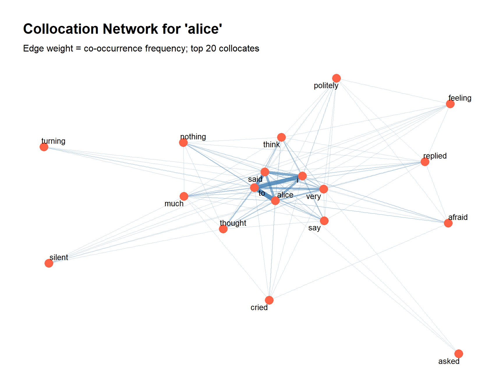
library(ggraph) library(igraph) # Get top 20 collocates and build a co-occurrence matrix for them top_colls <- alice_colls |> dplyr::arrange(dplyr::desc(phi)) |>head(20) |> dplyr::pull(w2) # Build FCM restricted to alice + its top collocates coll_network_data <- alice_sentences |> quanteda::tokens() |> quanteda::dfm() |> quanteda::dfm_select(pattern =c("alice", top_colls)) |> quanteda::fcm(tri =FALSE) # Convert to igraph for ggraph net <- igraph::graph_from_adjacency_matrix( as.matrix(coll_network_data), mode ="undirected", weighted =TRUE, diag =FALSE) # Plot ggraph::ggraph(net, layout ="fr") + ggraph::geom_edge_link(aes(width = weight, alpha = weight), colour ="steelblue") + ggraph::geom_node_point(colour ="tomato", size =5) + ggraph::geom_node_text(aes(label = name), repel =TRUE, size =3.5) + ggraph::scale_edge_width(range =c(0.3, 2.5)) + ggraph::scale_edge_alpha(range =c(0.3, 0.9)) +labs( title ="Collocation Network for 'alice'", subtitle ="Edge weight = co-occurrence frequency; top 20 collocates" ) +theme_graph() +theme(legend.position ="none")
The network plot reveals the semantic neighbourhood of alice in the novel: her characteristic actions (said, thought, went), the characters she interacts with (queen, king, cat, rabbit), and the emotions associated with her (poor).
Exercises: Collocation Analysis
Q1. What does it mean when O11 >> E11 in a collocation analysis?
Q2. Why is Mutual Information (MI) biased toward rare words, and what is the practical implication?
Keyword Analysis
Section Overview
What you’ll learn: How to identify words that are statistically over-represented in one corpus compared to a reference corpus — the method of keyword analysis
When to use it: When you want to characterise what makes one text or corpus distinctive; for comparing genres, authors, time periods, or groups
Keyword analysis identifies words that are key — statistically over-represented in a target corpus compared to a reference corpus. A keyword is not just a frequent word; it is a word whose frequency in the target corpus cannot be explained by its base rate in language generally (as captured by the reference corpus). Keywords characterise what is unusual, distinctive, or topically specific about a text.
The Keyword Analysis Logic
Like collocation analysis, keyword analysis uses a contingency table:
Target corpus
Reference corpus
Word present
O₁₁
O₁₂
Other words
O₂₁
O₂₂
The null hypothesis is that the word’s relative frequency is the same in both corpora. Statistical tests (log-likelihood, chi-square, Fisher’s exact test) evaluate whether the observed difference is larger than expected by chance.
Setting Up: Target and Reference Corpora
Code
# We will compare two chapters of Alice as a simple example
# Target: Chapter 8 (the Queen's croquet ground — "Off with their heads!")
# Reference: all other chapters combined

# Identify which chapters are which
cat("Chapter 8 begins:", substr(alice_chapters[9], 1, 80), "\n")
Chapter 8 begins: chapter viii. the queen’s croquet-ground a large rose-tree stood near the entran
Code
# Target: chapter 9 (index 9 = chapter 8 after the preamble) target_text <- alice_chapters[9] # Reference: all other chapters reference_text <-paste(alice_chapters[-9], collapse =" ") # Create a two-document corpus with a grouping variable kw_corpus <- quanteda::corpus( c(target_text, reference_text) ) docvars(kw_corpus, "group") <-c("target", "reference")
Computing Keyness
Code
# Build DFM grouped by target vs reference kw_dfm <- kw_corpus |> quanteda::tokens(remove_punct =TRUE) |> quanteda::dfm() |> quanteda::dfm_group(groups = group) # Compute keyness using log-likelihood (G2) — recommended for keyword analysis kw_results <- quanteda.textstats::textstat_keyness( x = kw_dfm, target ="target", measure ="lr"# log-likelihood ratio (G2) )
feature
G2
p
n_target
n_reference
queen
60.3609
0.0000
31
37
soldiers
32.0409
0.0000
9
1
gardeners
31.8253
0.0000
8
0
hedgehog
27.2322
0.0000
7
0
five
23.3106
0.0000
7
1
executioner
18.1234
0.0000
5
0
procession
18.1234
0.0000
5
0
three
17.6428
0.0000
11
15
game
15.2687
0.0001
7
5
seven
14.8236
0.0001
5
1
rose-tree
13.6309
0.0002
4
0
queen’s
12.6444
0.0004
5
2
flamingo
10.7339
0.0011
4
1
shouted
9.6871
0.0019
5
4
beheaded
9.2133
0.0024
3
0
Visualising Keywords
quanteda.textplots provides a dedicated plot for keyword results:
Code
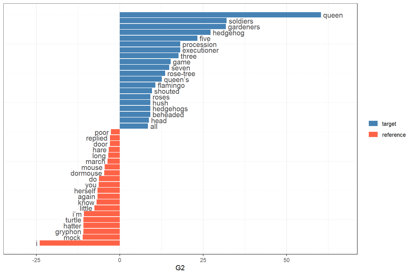
quanteda.textplots::textplot_keyness( x = kw_results, n =20, # show top 20 on each side color =c("steelblue", "tomato"), # positive / negative keywords show_reference =TRUE)
The plot shows:
Blue bars (left): Keywords — words over-represented in the target chapter
Red bars (right): Negative keywords — words over-represented in the reference (the rest of the novel)
Bar length: Keyness score (log-likelihood G²)
Computing tf-idf
An alternative to log-likelihood keyness is tf-idf weighting, which assigns each word a score reflecting how characteristic it is of each document within the collection:
Code
# Build raw count DFM with one document per chapterchapter_dfm <- quanteda::corpus(alice_chapters) |> quanteda::tokens(remove_punct =TRUE) |> quanteda::dfm()# Apply tf-idf weighting to the raw count DFMtfidf_dfm <- quanteda::dfm_tfidf(chapter_dfm,scheme_tf ="count",scheme_df ="inverse")# Extract top 15 most characteristic words for chapter 9# Convert to a tidy data frame manually — one row per feature per documentchapter9_tfidf <- tfidf_dfm[9, ] |># select chapter 9 row quanteda::convert(to ="data.frame") |># wide → data frame tidyr::pivot_longer(-doc_id,names_to ="feature",values_to ="tfidf") |># wide → long dplyr::filter(tfidf >0) |> dplyr::arrange(dplyr::desc(tfidf)) |>head(15)
feature
tf-idf score
chapter
queen
10.409555
text9
gardeners
8.911547
text9
hedgehog
7.797603
text9
soldiers
7.316220
text9
the
5.840034
text9
five
5.690393
text9
king
5.630717
text9
procession
5.569717
text9
executioner
5.569717
text9
rose-tree
4.455773
text9
seven
4.064567
text9
cat
3.734760
text9
Log-Likelihood vs. tf-idf: When to Use Each
Log-likelihood (G²) compares a target to a specific reference corpus using a significance test. It answers: Is this word’s frequency in my target significantly higher than in my reference? It is the standard method in corpus linguistics keyword analysis and is recommended when you have a clear comparison corpus.
tf-idf computes a weighting for each word in each document relative to the whole collection. It is most useful for information retrieval (finding the most characteristic terms in each document in a collection) and feature extraction for text classification. It does not require a separate reference corpus but is not directly interpretable as a significance test.
For most text analysis research questions (what makes text A distinctive compared to text B?), log-likelihood is the more appropriate method.
Exercises: Keyword Analysis
Q1. Why is the choice of reference corpus critical for keyword analysis?
Q2. A keyword analysis returns the, and, and of as the top keywords (with very high G² scores). What likely caused this, and how should it be addressed?
Quick Reference
Section Overview
A compact reference for the most commonly used functions and workflows in this tutorial
Martin Schweinberger. 2026. Introduction to Text Analysis: Practical Implementation in R. The Language Technology and Data Analysis Laboratory (LADAL), The University of Queensland, Australia. url: https://ladal.edu.au/tutorials/textanalysis/textanalysis.html (Version 3.1.1). doi: 10.5281/zenodo.19332976.
@manual{martinschweinberger2026introduction,
  author       = {Martin Schweinberger},
  title        = {Introduction to Text Analysis: Practical Implementation in R},
  year         = {2026},
  note         = {https://ladal.edu.au/tutorials/textanalysis/textanalysis.html},
  organization = {The Language Technology and Data Analysis Laboratory (LADAL), The University of Queensland, Australia},
  edition      = {3.1.1}
  doi      = {10.5281/zenodo.19332976}
}
This tutorial was re-developed with the assistance of Claude (claude.ai), a large language model created by Anthropic. Claude was used to help revise the tutorial text, structure the instructional content, generate the R code examples, and write the checkdown quiz questions and feedback strings. All content was reviewed, edited, and approved by the author (Martin Schweinberger), who takes full responsibility for the accuracy and pedagogical appropriateness of the material. The use of AI assistance is disclosed here in the interest of transparency and in accordance with emerging best practices for AI-assisted academic content creation.