Code
# Run once — comment out after installation
install.packages("tidyverse")
install.packages("flextable")
install.packages("ggforce")
install.packages("scales")
This tutorial demonstrates how to create personalised vowel charts using Praat and R. Vowel charts are among the most informative visualisations in phonetics and language learning: they map the acoustic properties of vowel sounds onto a two-dimensional space that closely mirrors the articulatory position of the tongue during vowel production.

The tutorial is aimed at beginners and intermediate users of R with an interest in phonetics, second language acquisition, or corpus phonology. It walks through the full workflow from recording to visualisation: recording words in Praat, extracting formant values, loading and processing the data in R, and producing publication-quality vowel charts with ggplot2. We also introduce vowel normalisation — an essential step when comparing speakers of different ages, sexes, or vocal tract sizes.
The aim is not to provide a fully-fledged acoustic analysis but to give a practical, step-by-step guide to vowel chart production that can be adapted for teaching and research purposes.
Before working through this tutorial, you should be familiar with:
Martin Schweinberger. 2026. Creating Vowel Charts in R. The Language Technology and Data Analysis Laboratory (LADAL), The University of Queensland, Australia. url: https://ladal.edu.au/tutorials/vowelchart/vowelchart.html (Version 3.1.1). doi: 10.5281/zenodo.19332987 .
# Run once — comment out after installation
install.packages("tidyverse")
install.packages("flextable")
install.packages("ggforce")
install.packages("scales")library(tidyverse)
library(flextable)
library(ggforce)
library(scales)
klippy::klippy()What you will learn: How vowels differ from consonants; what formants are and why F1 and F2 map onto the vowel space; and how a vowel chart relates to articulatory and acoustic phonetics
When learning or studying a language, one of the first distinctions encountered is that between consonants and vowels (Rogers 2014). Consonants are produced with an obstruction of the airstream; they cannot form the nucleus of a syllable on their own. Vowels, by contrast, are produced with an open, unobstructed vocal tract and form the carrying core of syllables (Zsiga 2012).
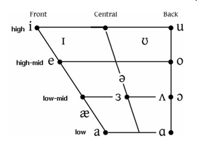
Because vowels are produced without obstruction, they are classified by different criteria than consonants:
The classical IPA vowel quadrilateral maps these articulatory dimensions onto a two-dimensional chart — the standard representation of the vowel space. Below is the chart for monophthongal vowels of Received Pronunciation (RP).
Vowels are periodic sounds — rhythmic compressions and decompressions of air produced by the vibration of the vocal folds. Each vowel is a complex periodic wave that can be decomposed into multiple simple periodic waves (formants) through acoustic analysis (Johnson 2003; Ladefoged 1996).
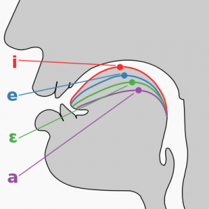
Formants are resonant frequency bands produced by the shape of the vocal tract. Different vowels are associated with different vocal tract shapes and therefore different formant patterns. The first two formants are linguistically the most important:
Formant | Articulatory correlate | Typical range (adult) |
|---|---|---|
F1 (first formant) | Tongue height — low vowels have high F1; high vowels have low F1 | 250–900 Hz |
F2 (second formant) | Tongue backness + lip rounding — front vowels have high F2; back/rounded vowels have low F2 | 700–2,500 Hz |
F3 (third formant) | Lip rounding and individual voice quality — less used in vowel classification | 1,700–3,500 Hz |
The key insight that makes acoustic vowel charts possible is that plotting F1 (y-axis, reversed) against F2 (x-axis, reversed) produces a display that closely mirrors the traditional articulatory vowel quadrilateral — high front vowels appear in the top-left, low back vowels in the bottom-right (Peterson and Barney 1952). This means that acoustic measurements from audio recordings can be used to produce a personalised vowel chart without needing to image the speaker’s tongue directly.
In a traditional vowel quadrilateral, high vowels are at the top and front vowels are on the left. Because F1 increases as the tongue lowers (low vowels = high F1), the y-axis is reversed so that low F1 (= high vowel) appears at the top. Similarly, F2 increases as the tongue moves forward (front vowels = high F2), so the x-axis is reversed so that high F2 (= front vowel) appears on the left. Reversing both axes aligns the acoustic plot with the traditional articulatory chart.
What you will learn: How to record words in Praat; how to set formant parameters; how to use TextGrids for reproducible annotation; how to extract F1 and F2 values; and an introduction to automated extraction via Praat scripting
To produce a vowel chart, we need recordings of words containing each monophthongal vowel sound. The standard approach uses minimal pairs in a controlled phonetic environment — typically the /h_d/ frame, which places vowels between two consonants with minimal coarticulation effects.
Word | IPA | Phonemic context | Vowel class |
|---|---|---|---|
had | æ | h _ d | low front |
hard | ɑ | h _ d | low back |
head | e | h _ d | mid front |
heed | i | h _ d | high front |
herd | ɜ | h _ d | mid central |
hid | ɪ | h _ d | high front lax |
hoard | ɔ | h _ d | mid back rounded |
hod | ɒ | h _ d | low back rounded |
hood | ʊ | h _ d | high back lax |
hud | ʌ | h _ d | mid central low |
who'd | u | h _ d | high back |
Each word should be repeated at least three times to allow for averaging across tokens, which reduces measurement error. Aim for a natural speaking rate — neither too fast nor too slow.
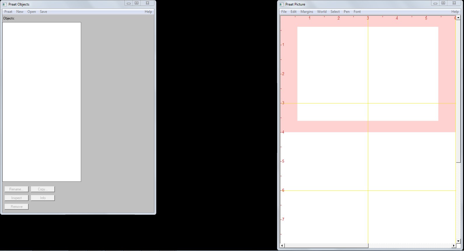
Download Praat from www.praat.org and install it. After installation:
vowels) in the Name field, and click Save to list & close.Microphone quality substantially affects formant accuracy. For research purposes, use a headset or close-talking microphone in a quiet room. For pedagogical purposes — e.g. giving a learner feedback on their vowel production — a laptop microphone in a reasonably quiet room is sufficient. Avoid recording near fans, air conditioning, or open windows.
Before extracting formants, the formant parameters must be set appropriately for the speaker:
If the formant dots in the edit window are scattered or erratic rather than forming smooth horizontal lines, try adjusting the Maximum formant setting up or down by 500 Hz, or change the Number of formants between 4 and 6. Poor tracking is most common in low back vowels where F1 and F2 are close together.
For each vowel token:
Record all values in a table. A completed table for one speaker is shown in the Data section below.
For research purposes, manual note-taking is not recommended — it is slow, error-prone, and not reproducible. TextGrids provide a structured, reusable annotation layer attached to the audio file.
To create a TextGrid:
vowel and a point tier named labelvowel tier and label each interval with the IPA symbol or wordOnce annotated, formants can be extracted for all labelled intervals using a Praat script, which eliminates the need to measure each token manually.
The following Praat script extracts the mean F1 and F2 from the midpoint of each labelled TextGrid interval and writes the results to a tab-delimited text file. Save this as extract_formants.praat and run it from Praat → Open Praat script.
# extract_formants.praat
# Extracts mean F1 and F2 from TextGrid interval midpoints
# Output: tab-delimited text file

form Extract formant values
  sentence Sound_file vowels.wav
  sentence TextGrid_file vowels.TextGrid
  real Maximum_formant_(Hz) 5500
  integer Number_of_formants 5
  sentence Output_file formants_output.txt
endform

Read from file: sound_file$
sound = selected("Sound")
Read from file: textGrid_file$
tg = selected("TextGrid")

# Create formant object
selectObject: sound
To Formant (burg): 0, number_of_formants, maximum_formant, 0.025, 50
formant = selected("Formant")

# Open output file
writeFileLine: output_file$, "label", tab$, "time", tab$, "F1", tab$, "F2"

# Loop over all intervals in tier 1
selectObject: tg
n = Get number of intervals: 1

for i from 1 to n
  label$ = Get label of interval: 1, i
  if label$ <> ""
    t_start = Get start time of interval: 1, i
    t_end   = Get end time of interval:   1, i
    t_mid   = (t_start + t_end) / 2

    selectObject: formant
    f1 = Get value at time: 1, t_mid, "Hertz", "Linear"
    f2 = Get value at time: 2, t_mid, "Hertz", "Linear"

    appendFileLine: output_file$,
      ... label$, tab$, fixed$(t_mid, 3), tab$,
      ... fixed$(f1, 2), tab$, fixed$(f2, 2)

    selectObject: tg
  endif
endfor

writeInfoLine: "Done! Output written to: ", output_file$A Praat script makes the measurement process reproducible (anyone can re-run it on the same audio and get the same values), scalable (it works equally well for 10 or 10,000 tokens), and consistent (all measurements are taken at the same relative position within each interval). For any analysis beyond a personal demonstration, scripted extraction is strongly preferred over manual measurement.
What you will learn: How to load and inspect formant data; how to combine a learner’s data with a native-speaker reference; how to compute mean formant values by vowel and speaker; and how to prepare the data for plotting
For this showcase we use two datasets:
nns — formant measurements from one L1-German learner of English, recorded using the /h_d/ word list and measured manually in Praatns — reference formant values for Received Pronunciation from Hawkins and Midgley (2005), representing five L1-RP speakers aged 20–25ns <- read.table("tutorials/vowelchart/data/rpvowels.txt", header = TRUE, sep = "\t")
nns <- read.table("tutorials/vowelchart/data/vowels.txt", header = TRUE, sep = "\t") |>
dplyr::select(-file)The learner data contains three repetitions of each word. Let us inspect the first few rows:
subject | item | trial | F1 | F2 |
|---|---|---|---|---|
ms | had | 1 | 717.3 | 1,868 |
ms | had | 2 | 743.5 | 1,904 |
ms | had | 3 | 721.0 | 1,939 |
ms | hard | 1 | 734.5 | 1,493 |
ms | hard | 2 | 832.9 | 1,408 |
ms | hard | 3 | 797.3 | 1,498 |
ms | head | 1 | 610.9 | 2,063 |
ms | head | 2 | 722.3 | 2,131 |
ms | head | 3 | 625.1 | 2,010 |
ms | heed | 1 | 263.4 | 2,833 |
ms | heed | 2 | 301.4 | 2,746 |
ms | heed | 3 | 287.0 | 2,823 |
The native-speaker reference data contains one row per vowel — the mean F1 and F2 across all speakers and tokens, plus standard deviations:
subject | item | trial | F1 | F2 |
|---|---|---|---|---|
S4-1 | heed | 1 | 261 | 2,282 |
S4-1 | heed | 2 | 288 | 2,304 |
S4-1 | heed | 3 | 307 | 2,373 |
S4-1 | heed | 4 | 328 | 2,416 |
S4-2 | heed | 1 | 290 | 2,215 |
S4-2 | heed | 2 | 257 | 2,263 |
S4-2 | heed | 3 | 290 | 2,255 |
S4-2 | heed | 4 | 251 | 2,223 |
S4-3 | heed | 1 | 235 | 2,552 |
S4-3 | heed | 2 | 270 | 2,479 |
S4-3 | heed | 3 | 238 | 2,434 |
S4-3 | heed | 4 | 295 | 2,459 |
S4-4 | heed | 1 | 295 | 1,962 |
S4-4 | heed | 2 | 291 | 1,996 |
S4-4 | heed | 3 | 309 | 1,983 |
S4-4 | heed | 4 | 269 | 2,045 |
S4-5 | heed | 1 | 244 | 2,632 |
S4-5 | heed | 2 | 268 | 2,640 |
S4-5 | heed | 3 | 284 | 2,627 |
S4-5 | heed | 4 | 253 | 2,612 |
S4-1 | hid | 1 | 454 | 2,375 |
S4-1 | hid | 2 | 452 | 2,032 |
S4-1 | hid | 3 | 424 | 2,003 |
S4-1 | hid | 4 | 441 | 2,098 |
S4-2 | hid | 1 | 368 | 2,105 |
S4-2 | hid | 2 | 345 | 2,089 |
S4-2 | hid | 3 | 338 | 2,161 |
S4-2 | hid | 4 | 390 | 2,079 |
S4-3 | hid | 1 | 378 | 2,438 |
S4-3 | hid | 2 | 411 | 2,369 |
S4-3 | hid | 3 | 421 | 2,360 |
S4-3 | hid | 4 | 366 | 2,442 |
S4-4 | hid | 1 | 346 | 2,000 |
S4-4 | hid | 2 | 342 | 1,974 |
S4-4 | hid | 3 | 374 | 1,930 |
S4-4 | hid | 4 | 335 | 1,996 |
S4-5 | hid | 1 | 414 | 2,311 |
S4-5 | hid | 2 | 454 | 2,256 |
S4-5 | hid | 3 | 389 | 2,278 |
S4-5 | hid | 4 | 415 | 2,191 |
S4-1 | head | 1 | 652 | 1,811 |
S4-1 | head | 2 | 638 | 1,838 |
S4-1 | head | 3 | 656 | 2,006 |
S4-1 | head | 4 | 547 | 1,960 |
S4-2 | head | 1 | 509 | 1,795 |
S4-2 | head | 2 | 409 | 1,845 |
S4-2 | head | 3 | 563 | 2,023 |
S4-2 | head | 4 | 473 | 1,979 |
S4-3 | head | 1 | 609 | 2,097 |
S4-3 | head | 2 | 721 | 2,130 |
S4-3 | head | 3 | 720 | 2,191 |
S4-3 | head | 4 | 706 | 1,950 |
S4-4 | head | 1 | 518 | 1,677 |
S4-4 | head | 2 | 444 | 1,985 |
S4-4 | head | 3 | 523 | 1,694 |
S4-4 | head | 4 | 515 | 1,726 |
S4-5 | head | 1 | 682 | 1,862 |
S4-5 | head | 2 | 737 | 1,912 |
S4-5 | head | 3 | 704 | 1,963 |
S4-5 | head | 4 | 673 | 2,070 |
S4-1 | had | 1 | 821 | 1,493 |
S4-1 | had | 2 | 845 | 1,458 |
S4-1 | had | 3 | 713 | 1,431 |
S4-1 | had | 4 | 875 | 1,470 |
S4-2 | had | 1 | 889 | 1,472 |
S4-2 | had | 2 | 805 | 1,379 |
S4-2 | had | 3 | 755 | 1,413 |
S4-2 | had | 4 | 839 | 1,345 |
S4-3 | had | 1 | 1,121 | 1,712 |
S4-3 | had | 2 | 1,021 | 1,578 |
S4-3 | had | 3 | 1,113 | 1,724 |
S4-3 | had | 4 | 1,127 | 1,695 |
S4-4 | had | 1 | 963 | 1,370 |
S4-4 | had | 2 | 1,049 | 1,459 |
S4-4 | had | 3 | 956 | 1,292 |
S4-4 | had | 4 | 1,009 | 1,396 |
S4-5 | had | 1 | 786 | 1,375 |
S4-5 | had | 2 | 839 | 1,476 |
S4-5 | had | 3 | 931 | 1,468 |
S4-5 | had | 4 | 870 | 1,457 |
S4-1 | hard | 1 | 627 | 1,052 |
S4-1 | hard | 2 | 593 | 1,043 |
S4-1 | hard | 3 | 595 | 1,109 |
S4-1 | hard | 4 | 635 | 1,078 |
S4-2 | hard | 1 | 621 | 1,033 |
S4-2 | hard | 2 | 570 | 1,040 |
S4-2 | hard | 3 | 570 | 1,007 |
S4-2 | hard | 4 | 503 | 970 |
S4-3 | hard | 1 | 574 | 994 |
S4-3 | hard | 2 | 587 | 996 |
S4-3 | hard | 3 | 455 | 986 |
S4-3 | hard | 4 | 570 | 989 |
S4-4 | hard | 1 | 531 | 1,044 |
S4-4 | hard | 2 | 620 | 1,092 |
S4-4 | hard | 3 | 637 | 1,066 |
S4-4 | hard | 4 | 562 | 1,081 |
S4-5 | hard | 1 | 668 | 1,038 |
S4-5 | hard | 2 | 699 | 1,027 |
S4-5 | hard | 3 | 762 | 1,068 |
S4-5 | hard | 4 | 704 | 1,090 |
S4-1 | hod | 1 | 517 | 900 |
S4-1 | hod | 2 | 518 | 994 |
S4-1 | hod | 3 | 526 | 886 |
S4-1 | hod | 4 | 526 | 850 |
S4-2 | hod | 1 | 486 | 870 |
S4-2 | hod | 2 | 486 | 873 |
S4-2 | hod | 3 | 470 | 872 |
S4-2 | hod | 4 | 443 | 907 |
S4-3 | hod | 1 | 457 | 797 |
S4-3 | hod | 2 | 490 | 816 |
S4-3 | hod | 3 | 508 | 890 |
S4-3 | hod | 4 | 496 | 811 |
S4-4 | hod | 1 | 452 | 830 |
S4-4 | hod | 2 | 451 | 782 |
S4-4 | hod | 3 | 454 | 826 |
S4-4 | hod | 4 | 433 | 891 |
S4-5 | hod | 1 | 520 | 878 |
S4-5 | hod | 2 | 410 | 851 |
S4-5 | hod | 3 | 486 | 855 |
S4-5 | hod | 4 | 533 | 919 |
S4-1 | hoard | 1 | 405 | 629 |
S4-1 | hoard | 2 | 389 | 644 |
S4-1 | hoard | 3 | 400 | 583 |
S4-1 | hoard | 4 | 396 | 561 |
S4-2 | hoard | 1 | 368 | 619 |
S4-2 | hoard | 2 | 370 | 714 |
S4-2 | hoard | 3 | 360 | 632 |
S4-2 | hoard | 4 | 353 | 637 |
S4-3 | hoard | 1 | 324 | 524 |
S4-3 | hoard | 2 | 367 | 573 |
S4-3 | hoard | 3 | 381 | 614 |
S4-3 | hoard | 4 | 391 | 571 |
S4-4 | hoard | 1 | 386 | 654 |
S4-4 | hoard | 2 | 335 | 570 |
S4-4 | hoard | 3 | 452 | 535 |
S4-4 | hoard | 4 | 469 | 654 |
S4-5 | hoard | 1 | 369 | 755 |
S4-5 | hoard | 2 | 419 | 540 |
S4-5 | hoard | 3 | 445 | 753 |
S4-5 | hoard | 4 | 454 | 830 |
S4-1 | hood | 1 | 454 | 1,550 |
S4-1 | hood | 2 | 420 | 1,741 |
S4-1 | hood | 3 | 409 | 1,657 |
S4-1 | hood | 4 | 426 | 1,610 |
S4-2 | hood | 1 | 400 | 1,200 |
S4-2 | hood | 2 | 452 | 1,332 |
S4-2 | hood | 3 | 423 | 1,198 |
S4-2 | hood | 4 | 381 | 1,158 |
S4-3 | hood | 1 | 421 | 1,222 |
S4-3 | hood | 2 | 424 | 1,150 |
S4-3 | hood | 3 | 446 | 1,252 |
S4-3 | hood | 4 | 436 | 1,174 |
S4-4 | hood | 1 | 353 | 1,087 |
S4-4 | hood | 2 | 370 | 1,100 |
S4-4 | hood | 3 | 369 | 1,153 |
S4-4 | hood | 4 | 357 | 1,281 |
S4-5 | hood | 1 | 453 | 1,275 |
S4-5 | hood | 2 | 393 | 1,223 |
S4-5 | hood | 3 | 417 | 1,125 |
S4-5 | hood | 4 | 453 | 1,245 |
S4-1 | whod | 1 | 331 | 1,983 |
S4-1 | whod | 2 | 314 | 1,956 |
S4-1 | whod | 3 | 311 | 1,984 |
S4-1 | whod | 4 | 311 | 1,796 |
S4-2 | whod | 1 | 307 | 1,416 |
S4-2 | whod | 2 | 330 | 1,545 |
S4-2 | whod | 3 | 251 | 1,462 |
S4-2 | whod | 4 | 278 | 1,314 |
S4-3 | whod | 1 | 294 | 1,315 |
S4-3 | whod | 2 | 272 | 1,527 |
S4-3 | whod | 3 | 250 | 1,589 |
S4-3 | whod | 4 | 281 | 1,576 |
S4-4 | whod | 1 | 297 | 1,446 |
S4-4 | whod | 2 | 229 | 1,241 |
S4-4 | whod | 3 | 262 | 1,605 |
S4-4 | whod | 4 | 303 | 1,589 |
S4-5 | whod | 1 | 332 | 1,917 |
S4-5 | whod | 2 | 251 | 1,660 |
S4-5 | whod | 3 | 268 | 1,778 |
S4-5 | whod | 4 | 302 | 1,627 |
S4-1 | hud | 1 | 592 | 1,242 |
S4-1 | hud | 2 | 668 | 1,163 |
S4-1 | hud | 3 | 690 | 1,202 |
S4-1 | hud | 4 | 654 | 1,195 |
S4-2 | hud | 1 | 539 | 1,301 |
S4-2 | hud | 2 | 471 | 1,239 |
S4-2 | hud | 3 | 537 | 1,390 |
S4-2 | hud | 4 | 587 | 1,347 |
S4-3 | hud | 1 | 922 | 1,224 |
S4-3 | hud | 2 | 805 | 1,191 |
S4-3 | hud | 3 | 805 | 1,107 |
S4-3 | hud | 4 | 738 | 1,124 |
S4-4 | hud | 1 | 500 | 1,224 |
S4-4 | hud | 2 | 620 | 1,107 |
S4-4 | hud | 3 | 587 | 1,207 |
S4-4 | hud | 4 | 572 | 1,218 |
S4-5 | hud | 1 | 670 | 1,177 |
S4-5 | hud | 2 | 679 | 1,155 |
S4-5 | hud | 3 | 784 | 1,178 |
S4-5 | hud | 4 | 744 | 1,170 |
S4-1 | herd | 1 | 590 | 1,498 |
S4-1 | herd | 2 | 571 | 1,537 |
S4-1 | herd | 3 | 520 | 1,532 |
S4-1 | herd | 4 | 514 | 1,545 |
S4-2 | herd | 1 | 479 | 1,419 |
S4-2 | herd | 2 | 500 | 1,399 |
S4-2 | herd | 3 | 420 | 1,391 |
S4-2 | herd | 4 | 466 | 1,417 |
S4-3 | herd | 1 | 462 | 1,252 |
S4-3 | herd | 2 | 428 | 1,224 |
S4-3 | herd | 3 | 464 | 1,282 |
S4-3 | herd | 4 | 515 | 1,278 |
S4-4 | herd | 1 | 461 | 1,334 |
S4-4 | herd | 2 | 449 | 1,273 |
S4-4 | herd | 3 | 431 | 1,347 |
S4-4 | herd | 4 | 486 | 1,344 |
S4-5 | herd | 1 | 537 | 1,366 |
S4-5 | herd | 2 | 499 | 1,364 |
S4-5 | herd | 3 | 533 | 1,314 |
S4-5 | herd | 4 | 546 | 1,332 |
We first combine the two datasets and rename the key columns:
voweldata <- rbind(nns, ns) |>
  dplyr::rename(Speaker = subject, Word = item) |>
  dplyr::mutate(
    Speaker = dplyr::case_when(
      Speaker == "ms"    ~ "L1-German learner",
      Speaker == "rpspk" ~ "RP native speakers",
      TRUE               ~ Speaker
    )
  )
Next we add IPA symbols for each word:
voweldata <- voweldata |>
  dplyr::mutate(
    ipa = dplyr::case_when(
      Word == "had"   ~ "\u00E6",
      Word == "hard"  ~ "\u0251",
      Word == "head"  ~ "e",
      Word == "heed"  ~ "i",
      Word == "herd"  ~ "\u025C",
      Word == "hid"   ~ "\u026A",
      Word == "hoard" ~ "\u0254",
      Word == "hod"   ~ "\u0252",
      Word == "hood"  ~ "\u028A",
      Word == "hud"   ~ "\u028C",
      Word == "whod"  ~ "u",
      TRUE            ~ "?"
    )
  )
Finally, we compute per-vowel mean F1 and F2 within each speaker group and drop the trial column:
voweldata <- voweldata |>
  dplyr::group_by(Speaker, Word) |>
  dplyr::mutate(
    F1_mean = mean(F1),
    F2_mean = mean(F2)
  ) |>
  dplyr::ungroup() |>
  dplyr::select(-dplyr::any_of("trial"))
The resulting table of per-vowel means looks like this:
Speaker | Word | ipa | F1_mean | F2_mean |
|---|---|---|---|---|
L1-German learner | had | æ | 727.3 | 1,903.5 |
L1-German learner | hard | ɑ | 788.2 | 1,466.5 |
L1-German learner | head | e | 652.8 | 2,067.7 |
L1-German learner | heed | i | 283.9 | 2,800.5 |
L1-German learner | herd | ɜ | 531.8 | 1,743.0 |
L1-German learner | hid | ɪ | 426.5 | 2,411.4 |
L1-German learner | hoard | ɔ | 579.4 | 990.5 |
L1-German learner | hod | ɒ | 688.2 | 1,227.8 |
L1-German learner | hood | ʊ | 435.2 | 1,382.5 |
L1-German learner | hud | ʌ | 672.6 | 1,597.4 |
L1-German learner | whod | u | 355.8 | 1,105.3 |
S4-1 | had | æ | 813.5 | 1,463.0 |
S4-1 | hard | ɑ | 612.5 | 1,070.5 |
S4-1 | head | e | 623.2 | 1,903.8 |
S4-1 | heed | i | 296.0 | 2,343.8 |
S4-1 | herd | ɜ | 548.8 | 1,528.0 |
S4-1 | hid | ɪ | 442.8 | 2,127.0 |
S4-1 | hoard | ɔ | 397.5 | 604.2 |
S4-1 | hod | ɒ | 521.8 | 907.5 |
S4-1 | hood | ʊ | 427.2 | 1,639.5 |
S4-1 | hud | ʌ | 651.0 | 1,200.5 |
S4-1 | whod | u | 316.8 | 1,929.8 |
S4-2 | had | æ | 822.0 | 1,402.2 |
S4-2 | hard | ɑ | 566.0 | 1,012.5 |
S4-2 | head | e | 488.5 | 1,910.5 |
S4-2 | heed | i | 272.0 | 2,239.0 |
S4-2 | herd | ɜ | 466.2 | 1,406.5 |
S4-2 | hid | ɪ | 360.2 | 2,108.5 |
S4-2 | hoard | ɔ | 362.8 | 650.5 |
S4-2 | hod | ɒ | 471.2 | 880.5 |
S4-2 | hood | ʊ | 414.0 | 1,222.0 |
S4-2 | hud | ʌ | 533.5 | 1,319.2 |
S4-2 | whod | u | 291.5 | 1,434.2 |
S4-3 | had | æ | 1,095.5 | 1,677.2 |
S4-3 | hard | ɑ | 546.5 | 991.2 |
S4-3 | head | e | 689.0 | 2,092.0 |
S4-3 | heed | i | 259.5 | 2,481.0 |
S4-3 | herd | ɜ | 467.2 | 1,259.0 |
S4-3 | hid | ɪ | 394.0 | 2,402.2 |
S4-3 | hoard | ɔ | 365.8 | 570.5 |
S4-3 | hod | ɒ | 487.8 | 828.5 |
S4-3 | hood | ʊ | 431.8 | 1,199.5 |
S4-3 | hud | ʌ | 817.5 | 1,161.5 |
S4-3 | whod | u | 274.2 | 1,501.8 |
S4-4 | had | æ | 994.2 | 1,379.2 |
S4-4 | hard | ɑ | 587.5 | 1,070.8 |
S4-4 | head | e | 500.0 | 1,770.5 |
S4-4 | heed | i | 291.0 | 1,996.5 |
S4-4 | herd | ɜ | 456.8 | 1,324.5 |
S4-4 | hid | ɪ | 349.2 | 1,975.0 |
S4-4 | hoard | ɔ | 410.5 | 603.2 |
S4-4 | hod | ɒ | 447.5 | 832.2 |
S4-4 | hood | ʊ | 362.2 | 1,155.2 |
S4-4 | hud | ʌ | 569.8 | 1,189.0 |
S4-4 | whod | u | 272.8 | 1,470.2 |
S4-5 | had | æ | 856.5 | 1,444.0 |
S4-5 | hard | ɑ | 708.2 | 1,055.8 |
S4-5 | head | e | 699.0 | 1,951.8 |
S4-5 | heed | i | 262.2 | 2,627.8 |
S4-5 | herd | ɜ | 528.8 | 1,344.0 |
S4-5 | hid | ɪ | 418.0 | 2,259.0 |
S4-5 | hoard | ɔ | 421.8 | 719.5 |
S4-5 | hod | ɒ | 487.2 | 875.8 |
S4-5 | hood | ʊ | 429.0 | 1,217.0 |
S4-5 | hud | ʌ | 719.2 | 1,170.0 |
S4-5 | whod | u | 288.2 | 1,745.5 |
What you will learn: Why raw formant values cannot always be compared across speakers; what Lobanov and Nearey normalisation are; how to apply both methods in R; and when each is appropriate
Raw formant values (in Hz) reflect both the vowel category and the speaker’s individual vocal tract size. Adult males have longer vocal tracts than females, who in turn have longer vocal tracts than children — this means that the same vowel produced by a male and a female speaker will have different Hz values even if both are native speakers of the same variety.
When comparing a single speaker to themselves over time or two speakers from the same demographic group (as in this showcase), the effect is modest and raw Hz values are often acceptable. However, when comparing speakers of different sexes, ages, or sizes — or when pooling across many speakers — normalisation is essential to separate linguistic (vowel category) variation from anatomical (vocal tract size) variation.
Method | Description | Best for |
|---|---|---|
Lobanov (z-score) | z-score each formant within each speaker: (F − mean) / SD | Cross-sex, cross-age comparison; large multi-speaker corpora |
Nearey (log-mean) | Subtract speaker's log-mean from log-transformed formants | Corpora where speaker means differ but variances are similar |
Bark scaling | Convert Hz to Bark scale using a perceptual transform | Perceptually motivated analyses |
Watt & Fabricius | Reference vowel triangle method — preserves relative distances | Dialect surveys; comparison of vowel system geometry |
Raw Hz (no normalisation) | No transformation — absolute Hz values retained | Single speaker; speakers matched for age and sex |
The Lobanov method z-scores each formant separately within each speaker — it is the most widely used method for cross-speaker comparison (Lobanov 1971):
\[F_{\text{Lobanov}} = \frac{F - \bar{F}_{\text{speaker}}}{SD_{F,\text{speaker}}}\]
We first compute the z-scored formant values:
voweldata_lob <- voweldata |>
  dplyr::group_by(Speaker) |>
  dplyr::mutate(
    F1_lob = (F1 - mean(F1, na.rm = TRUE)) / sd(F1, na.rm = TRUE),
    F2_lob = (F2 - mean(F2, na.rm = TRUE)) / sd(F2, na.rm = TRUE)
  ) |>
  dplyr::ungroup()
Then we add per-vowel means on the normalised scale:
voweldata_lob <- voweldata_lob |>
  dplyr::group_by(Speaker, Word) |>
  dplyr::mutate(
    F1_lob_mean = mean(F1_lob),
    F2_lob_mean = mean(F2_lob)
  ) |>
dplyr::ungroup()The Nearey method applies a log transformation and subtracts the speaker’s log-mean across all formants (Nearey 1989). It is less aggressive than Lobanov and preserves more of the relative distances between vowels:
\[F_{\text{Nearey}} = \log(F) - \frac{1}{n}\sum_{k=1}^{n}\overline{\log(F_k)}\]
We compute the log grand mean per speaker, then subtract it from each log-transformed formant:
voweldata_nea <- voweldata |>
  dplyr::group_by(Speaker) |>
  dplyr::mutate(
    log_grand_mean = mean(c(log(F1), log(F2)), na.rm = TRUE),
    F1_nea = log(F1) - log_grand_mean,
    F2_nea = log(F2) - log_grand_mean
  ) |>
  dplyr::ungroup()
Then we add per-vowel means on the Nearey scale:
voweldata_nea <- voweldata_nea |>
  dplyr::group_by(Speaker, Word) |>
  dplyr::mutate(
    F1_nea_mean = mean(F1_nea),
    F2_nea_mean = mean(F2_nea)
  ) |>
dplyr::ungroup()What you will learn: How to produce a basic vowel chart with ggplot2; how to add confidence ellipses; how to create a publication-quality comparison chart with native-speaker reference ellipses; and how to plot normalised vowel spaces
We first separate the two speaker groups so that we can apply different ellipse levels to each:
ns_data  <- voweldata |> dplyr::filter(Speaker == "RP native speakers")
nns_data <- voweldata |> dplyr::filter(Speaker == "L1-German learner")
We also prepare a deduplicated means table for the IPA label layer:
vowel_means <- voweldata |>
  dplyr::distinct(Speaker, Word, ipa, F1_mean, F2_mean)
Now we build the chart in layers — points, IPA labels, and ellipses — then apply the reversed axes and styling:
ggplot(voweldata,
aes(x = F2, y = F1, color = Speaker, fill = Speaker)) +
geom_point(alpha = 0.15, size = 1.5) +
geom_text(
data = vowel_means,
aes(x = F2_mean, y = F1_mean, label = ipa),
fontface = "bold", size = 4.5, show.legend = FALSE
) +
stat_ellipse(data = ns_data, level = 0.50, geom = "polygon",
alpha = 0.08, linetype = "dashed") +
stat_ellipse(data = nns_data, level = 0.95, geom = "polygon",
alpha = 0.08) +
scale_x_reverse(breaks = seq(500, 3000, 500)) +
scale_y_reverse(breaks = seq(200, 1000, 100)) +
scale_color_manual(values = c("L1-German learner" = "#E67E22",
"RP native speakers" = "#2C3E50")) +
scale_fill_manual(values = c("L1-German learner" = "#E67E22",
"RP native speakers" = "#2C3E50")) +
theme_bw() +
theme(
legend.position = "top",
legend.title = element_blank(),
panel.grid.major = element_blank(),
panel.grid.minor = element_blank(),
axis.title = element_text(size = 11)
) +
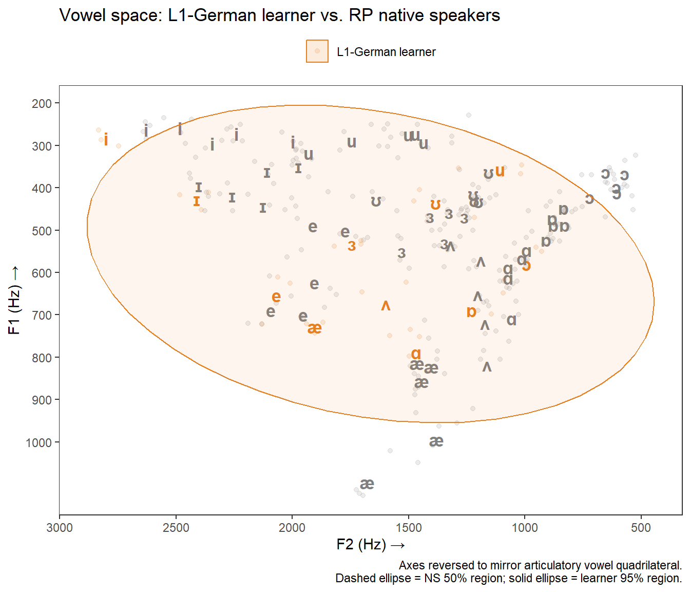
labs(
title = "Vowel space: L1-German learner vs. RP native speakers",
x = "F2 (Hz) →",
y = "F1 (Hz) →",
caption = "Axes reversed to mirror articulatory vowel quadrilateral.\nDashed ellipse = NS 50% region; solid ellipse = learner 95% region."
)
For the native-speaker reference data, we have standard deviations provided directly by Hawkins and Midgley (2005). We can use these to draw standard-deviation ellipses that represent the spread of the native-speaker vowel space more accurately than stat_ellipse().
We first prepare the native-speaker means data, adding IPA labels:
# Reference means and SDs from Hawkins & Midgley (2005)
# Five L1-RP speakers aged 20-25
ns_means <- data.frame(
  Word = c("had","hard","head","heed","herd","hid","hoard","hod","hood","hud","whod"),
  F1   = c(916.35, 604.15, 599.95, 276.15, 493.55, 392.85, 391.65, 483.10, 412.85, 658.20, 288.70),
  F2   = c(1473.15, 1040.15, 1925.70, 2337.60, 1372.40, 2174.35, 629.60, 864.90, 1286.65, 1208.05, 1616.30),
  F1sd = c(124.30, 70.92, 102.23, 25.48, 47.41, 40.84, 39.71, 35.48, 32.98, 116.15, 30.19),
  F2sd = c(119.44, 40.06, 143.60, 223.42, 95.95, 166.86, 81.19, 48.50, 193.70, 72.52, 225.74),
  ipa  = c("\u00E6", "\u0251", "e", "i", "\u025C", "\u026A",
           "\u0254", "\u0252", "\u028A", "\u028C", "u")
)
Next we extract the learner means and join them with the NS means to compute displacement arrows:
nns_means <- voweldata |>
  dplyr::filter(Speaker == "L1-German learner") |>
  dplyr::distinct(Word, ipa, F1_mean, F2_mean)

arrow_data <- dplyr::left_join(nns_means, ns_means, by = c("Word", "ipa"))
Now we build the chart with ggforce::geom_ellipse() for the SD ellipses and geom_segment() for the displacement arrows:
ggplot() +
  ggforce::geom_ellipse(
    data = ns_means,
    aes(x0 = F2, y0 = F1, a = F2sd, b = F1sd, angle = 0),
    fill = "#2C3E50", alpha = 0.07, color = "#2C3E50",
    linetype = "dashed", linewidth = 0.5
  ) +
  geom_text(
    data = ns_means,
    aes(x = F2, y = F1, label = ipa),
    color = "#2C3E50", fontface = "bold", size = 5
  ) +
  geom_text(
    data = nns_means,
    aes(x = F2_mean, y = F1_mean, label = ipa),
    color = "#E67E22", fontface = "bold", size = 5
  ) +
  geom_segment(
    data = arrow_data,
    aes(x = F2_mean, y = F1_mean, xend = F2, yend = F1),
    arrow = arrow(length = unit(0.15, "cm"), type = "closed"),
    color = "grey50", linewidth = 0.4, alpha = 0.7
  ) +
  scale_x_reverse(breaks = seq(500, 3000, 500),
                  labels = scales::label_number()) +
  scale_y_reverse(breaks = seq(200, 1000, 100)) +
  theme_bw() +
  theme(
    panel.grid.major = element_blank(),
    panel.grid.minor = element_blank(),
    axis.title       = element_text(size = 11),
    plot.caption     = element_text(size = 8, color = "grey40")
  ) +
  labs(
    title   = "Vowel space comparison: L1-German learner (orange) vs. RP native speakers (dark)",
    x       = "F2 (Hz) →",
    y       = "F1 (Hz) →",
    caption = "Dashed ellipses = ±1 SD of native RP speaker vowel spaces (Hawkins & Midgley 2005).\nArrows indicate direction and magnitude of learner deviation from native norms."
  )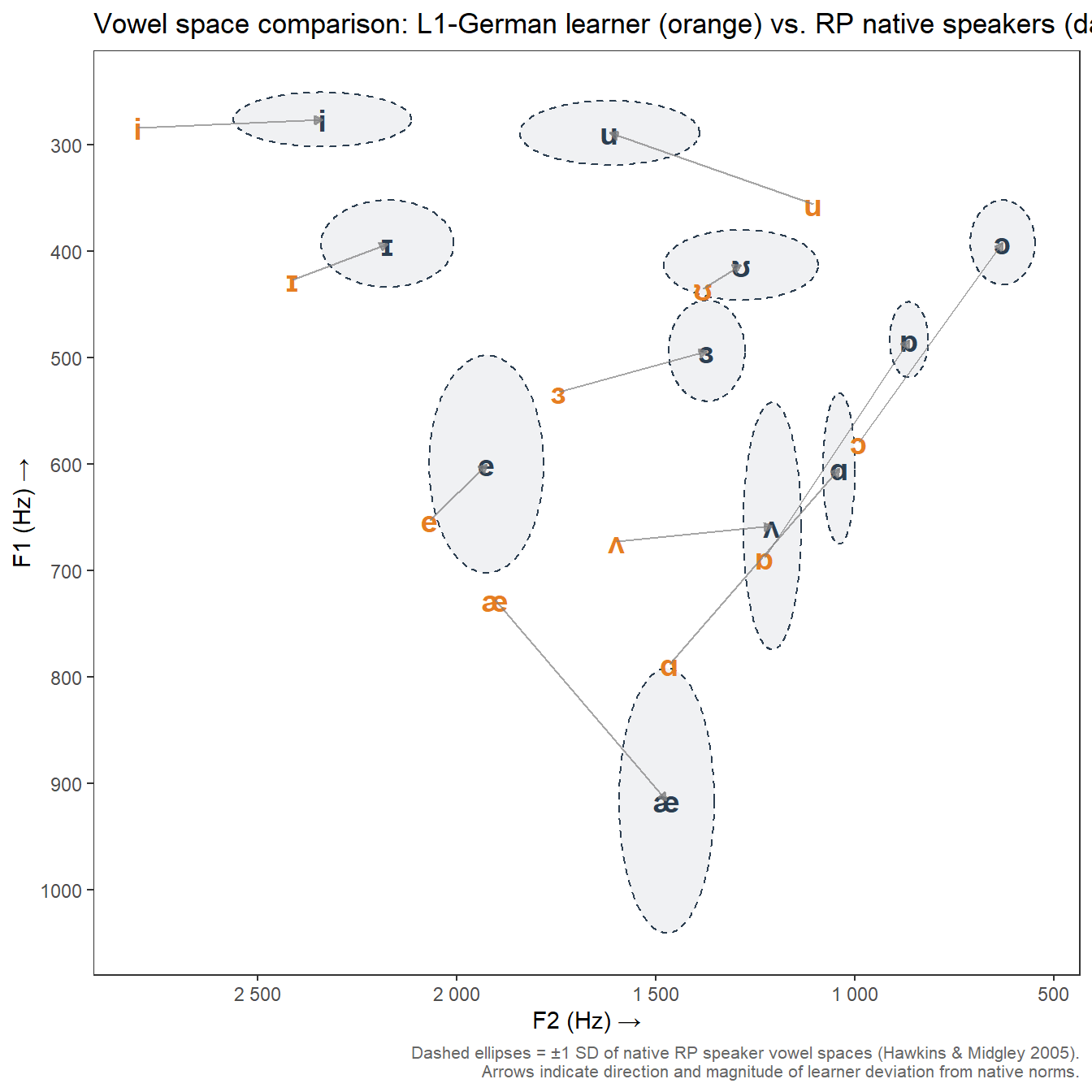
The arrows make displacement patterns immediately interpretable: vowels where the arrow is long indicate larger deviations from the native-speaker target. The chart shows that the L1-German learner’s /iː/ (heed) and /ɔː/ (hoard) are displaced most substantially from RP norms.
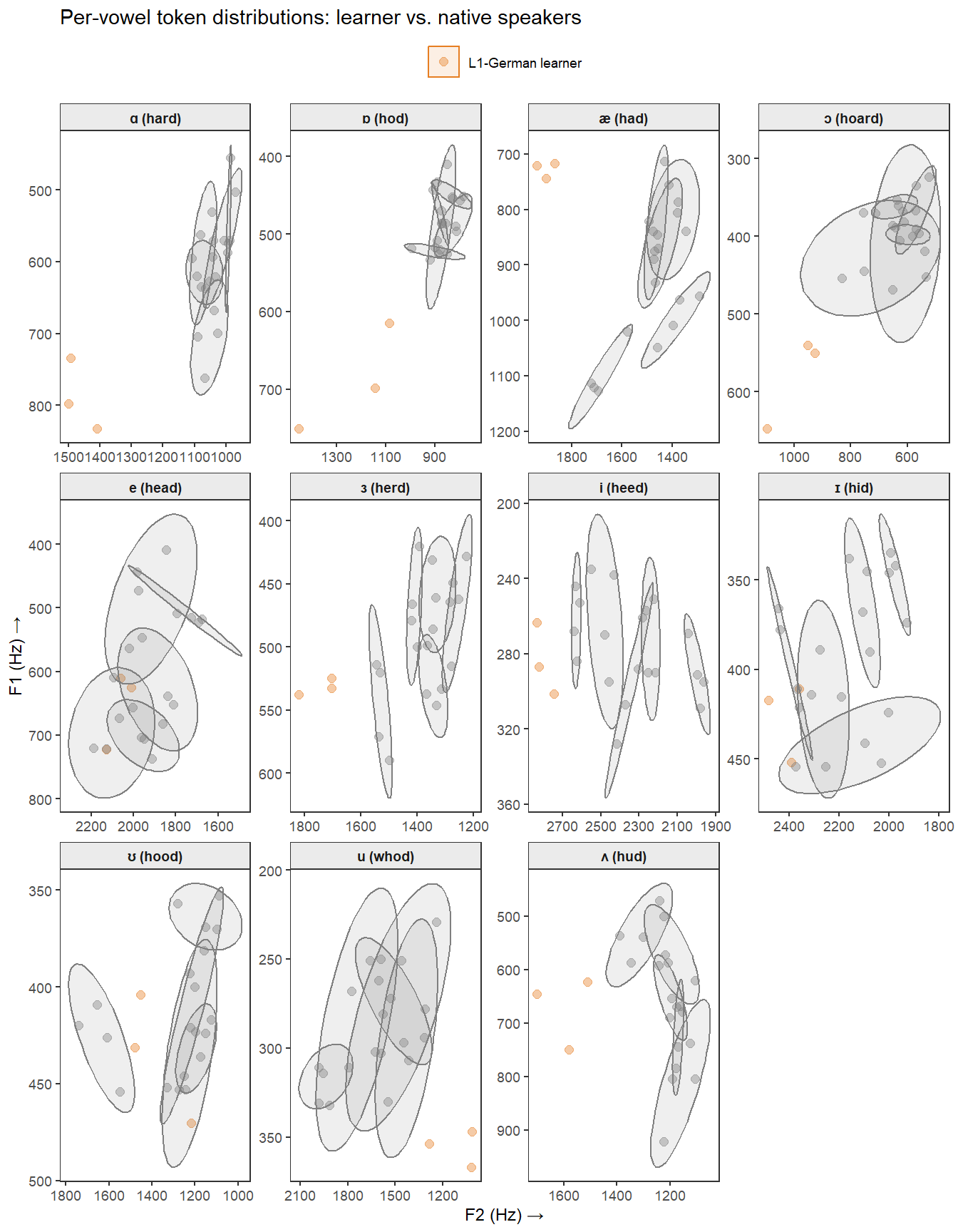
A faceted view allows close inspection of each vowel’s token distribution. We first filter out any rows with missing formant values, then pass the data to ggplot():
voweldata_clean <- voweldata |>
  dplyr::filter(!is.na(F1), !is.na(F2)) |>
dplyr::mutate(facet_label = paste0(ipa, " (", Word, ")"))ggplot(voweldata_clean,
aes(x = F2, y = F1, color = Speaker, fill = Speaker)) +
geom_point(alpha = 0.4, size = 2) +
stat_ellipse(level = 0.80, geom = "polygon", alpha = 0.12) +
facet_wrap(~ facet_label, ncol = 4, scales = "free") +
scale_x_reverse() +
scale_y_reverse() +
scale_color_manual(values = c("L1-German learner" = "#E67E22",
"RP native speakers" = "#2C3E50")) +
scale_fill_manual(values = c("L1-German learner" = "#E67E22",
"RP native speakers" = "#2C3E50")) +
theme_bw(base_size = 9) +
theme(
legend.position = "top",
legend.title = element_blank(),
panel.grid = element_blank(),
strip.background = element_rect(fill = "grey92"),
strip.text = element_text(face = "bold")
) +
labs(
title = "Per-vowel token distributions: learner vs. native speakers",
x = "F2 (Hz) →", y = "F1 (Hz) →"
)
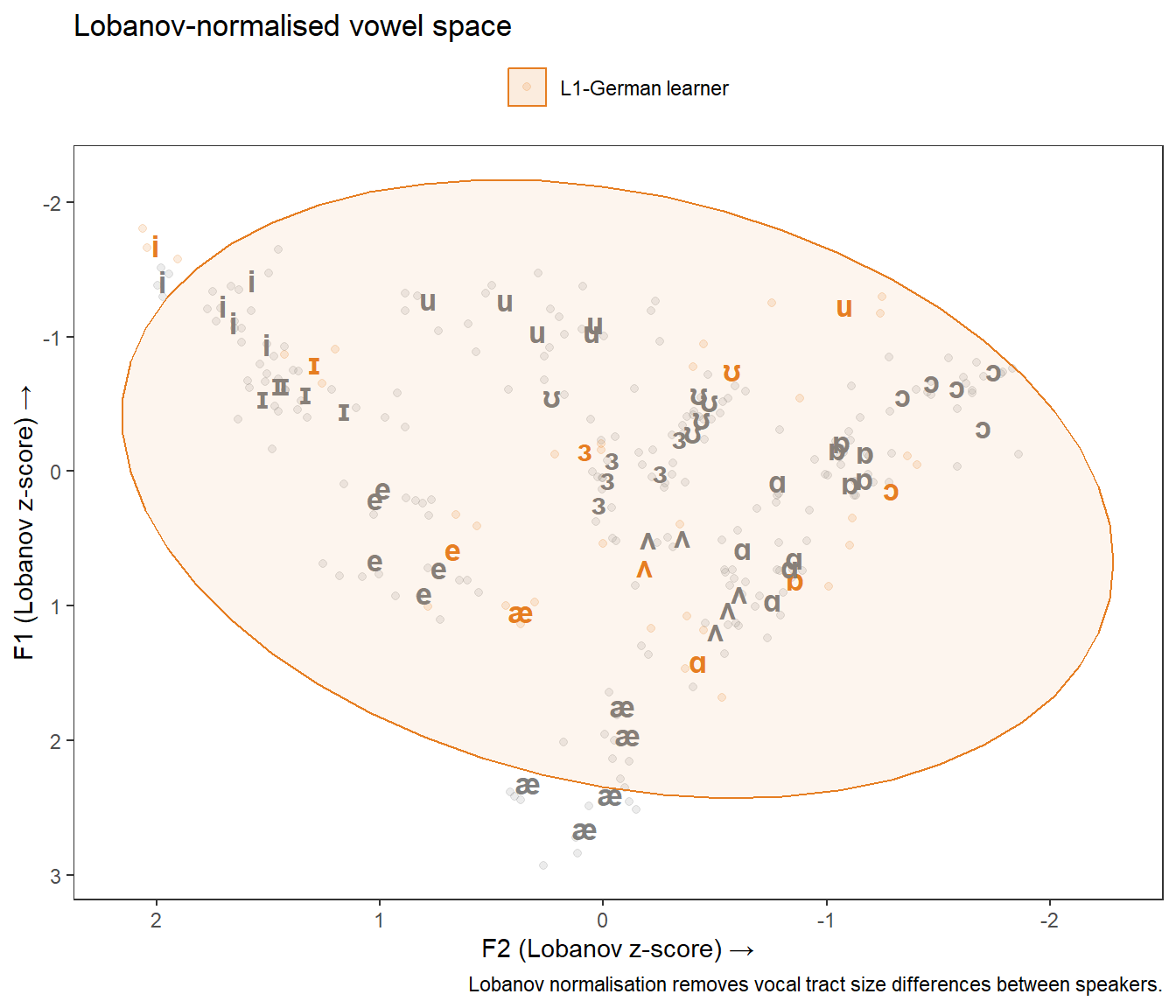
We first split the Lobanov-normalised data by speaker group:
ns_lob  <- voweldata_lob |> dplyr::filter(Speaker == "RP native speakers")
nns_lob <- voweldata_lob |> dplyr::filter(Speaker == "L1-German learner")

lob_means <- voweldata_lob |>
dplyr::distinct(Speaker, Word, ipa, F1_lob_mean, F2_lob_mean)ggplot(voweldata_lob,
aes(x = F2_lob, y = F1_lob, color = Speaker, fill = Speaker)) +
geom_point(alpha = 0.15, size = 1.5) +
geom_text(
data = lob_means,
aes(x = F2_lob_mean, y = F1_lob_mean, label = ipa),
fontface = "bold", size = 4.5, show.legend = FALSE
) +
stat_ellipse(data = ns_lob, level = 0.50, geom = "polygon",
alpha = 0.08, linetype = "dashed") +
stat_ellipse(data = nns_lob, level = 0.95, geom = "polygon",
alpha = 0.08) +
scale_x_reverse() +
scale_y_reverse() +
scale_color_manual(values = c("L1-German learner" = "#E67E22",
"RP native speakers" = "#2C3E50")) +
scale_fill_manual(values = c("L1-German learner" = "#E67E22",
"RP native speakers" = "#2C3E50")) +
theme_bw() +
theme(
legend.position = "top",
legend.title = element_blank(),
panel.grid = element_blank()
) +
labs(
title = "Lobanov-normalised vowel space",
x = "F2 (Lobanov z-score) →",
y = "F1 (Lobanov z-score) →",
caption = "Lobanov normalisation removes vocal tract size differences between speakers."
)
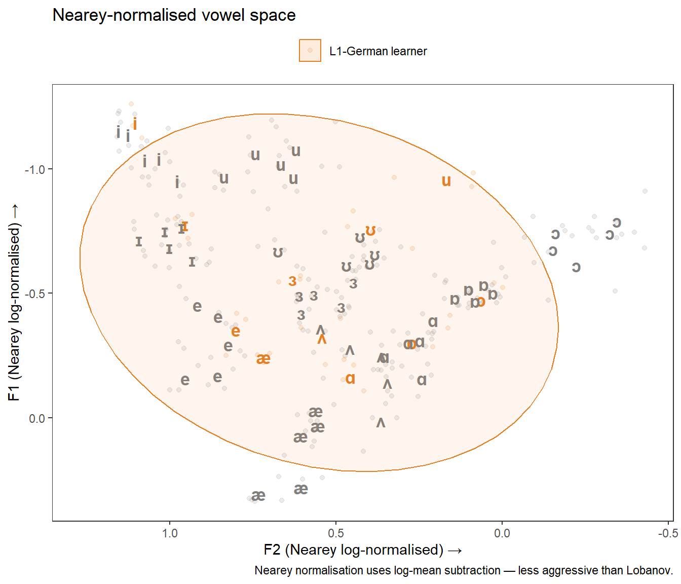
We do the same for the Nearey-normalised data:
ns_nea  <- voweldata_nea |> dplyr::filter(Speaker == "RP native speakers")
nns_nea <- voweldata_nea |> dplyr::filter(Speaker == "L1-German learner")

nea_means <- voweldata_nea |>
dplyr::distinct(Speaker, Word, ipa, F1_nea_mean, F2_nea_mean)ggplot(voweldata_nea,
aes(x = F2_nea, y = F1_nea, color = Speaker, fill = Speaker)) +
geom_point(alpha = 0.15, size = 1.5) +
geom_text(
data = nea_means,
aes(x = F2_nea_mean, y = F1_nea_mean, label = ipa),
fontface = "bold", size = 4.5, show.legend = FALSE
) +
stat_ellipse(data = ns_nea, level = 0.50, geom = "polygon",
alpha = 0.08, linetype = "dashed") +
stat_ellipse(data = nns_nea, level = 0.95, geom = "polygon",
alpha = 0.08) +
scale_x_reverse() +
scale_y_reverse() +
scale_color_manual(values = c("L1-German learner" = "#E67E22",
"RP native speakers" = "#2C3E50")) +
scale_fill_manual(values = c("L1-German learner" = "#E67E22",
"RP native speakers" = "#2C3E50")) +
theme_bw() +
theme(
legend.position = "top",
legend.title = element_blank(),
panel.grid = element_blank()
) +
labs(
title = "Nearey-normalised vowel space",
x = "F2 (Nearey log-normalised) →",
y = "F1 (Nearey log-normalised) →",
caption = "Nearey normalisation uses log-mean subtraction — less aggressive than Lobanov."
)
For a single-speaker showcase like this one, raw Hz values are perfectly adequate and most interpretable. For a study comparing speakers across sexes or ages, Lobanov is the standard choice in sociophonetics. Nearey is preferred when the absolute distances between vowels are theoretically important, as it is less aggressive. If in doubt, report both and note whether the substantive conclusions differ.
We assemble one row of means per speaker per vowel under each scheme, tag each with a normalisation label, and combine into a single data frame:
means_raw <- voweldata |>
  dplyr::distinct(Speaker, Word, ipa, F1_mean, F2_mean) |>
dplyr::mutate(normalisation = "Raw Hz")means_lob <- voweldata_lob |>
dplyr::distinct(Speaker, Word, ipa, F1_lob_mean, F2_lob_mean) |>
dplyr::rename(F1_mean = F1_lob_mean, F2_mean = F2_lob_mean) |>
dplyr::mutate(normalisation = "Lobanov")means_nea <- voweldata_nea |>
dplyr::distinct(Speaker, Word, ipa, F1_nea_mean, F2_nea_mean) |>
dplyr::rename(F1_mean = F1_nea_mean, F2_mean = F2_nea_mean) |>
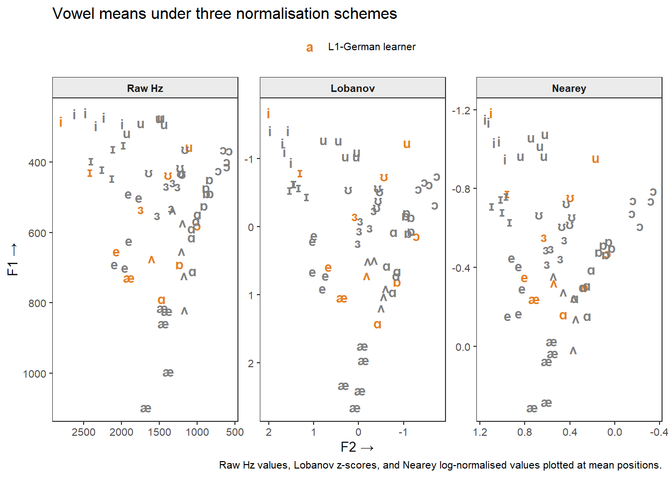
dplyr::mutate(normalisation = "Nearey")means_all <- dplyr::bind_rows(means_raw, means_lob, means_nea) |>
dplyr::mutate(normalisation = factor(normalisation,
levels = c("Raw Hz", "Lobanov", "Nearey")))ggplot(means_all,
aes(x = F2_mean, y = F1_mean, color = Speaker, label = ipa)) +
geom_text(fontface = "bold", size = 3.5) +
facet_wrap(~ normalisation, scales = "free") +
scale_x_reverse() +
scale_y_reverse() +
scale_color_manual(values = c("L1-German learner" = "#E67E22",
"RP native speakers" = "#2C3E50")) +
theme_bw(base_size = 10) +
theme(
legend.position = "top",
legend.title = element_blank(),
panel.grid = element_blank(),
strip.background = element_rect(fill = "grey92"),
strip.text = element_text(face = "bold")
) +
labs(
title = "Vowel means under three normalisation schemes",
x = "F2 →", y = "F1 →",
caption = "Raw Hz values, Lobanov z-scores, and Nearey log-normalised values plotted at mean positions."
)
The vowel charts reveal several patterns in the L1-German learner’s English vowel production relative to the RP native-speaker norms:
These observations are consistent with the broader SLA literature on L1-German speakers’ English phonology (see Paganus et al. 2006 for similar analyses in a language-learning feedback context).
Martin Schweinberger. 2026. Creating Vowel Charts in R. The Language Technology and Data Analysis Laboratory (LADAL), The University of Queensland, Australia. url: https://ladal.edu.au/tutorials/vowelchart/vowelchart.html (Version 3.1.1). doi: 10.5281/zenodo.19332987 .
@manual{martinschweinberger2026creating,
  author       = {Martin Schweinberger},
  title        = {Creating Vowel Charts in R},
  year         = {2026},
  note         = {https://ladal.edu.au/tutorials/vowelchart/vowelchart.html},
  organization = {The Language Technology and Data Analysis Laboratory (LADAL), The University of Queensland, Australia},
  edition      = {2026.03.27}
  doi      = {10.5281/zenodo.19242479}
}sessionInfo()R version 4.4.2 (2024-10-31 ucrt)
Platform: x86_64-w64-mingw32/x64
Running under: Windows 11 x64 (build 26200)
Matrix products: default
locale:
[1] LC_COLLATE=English_United States.utf8
[2] LC_CTYPE=English_United States.utf8
[3] LC_MONETARY=English_United States.utf8
[4] LC_NUMERIC=C
[5] LC_TIME=English_United States.utf8
time zone: Australia/Brisbane
tzcode source: internal
attached base packages:
[1] stats graphics grDevices datasets utils methods base
other attached packages:
[1] scales_1.4.0 ggforce_0.4.2 flextable_0.9.11 lubridate_1.9.4
[5] forcats_1.0.0 stringr_1.5.1 dplyr_1.2.0 purrr_1.0.4
[9] readr_2.1.5 tidyr_1.3.2 tibble_3.2.1 ggplot2_4.0.2
[13] tidyverse_2.0.0
loaded via a namespace (and not attached):
[1] gtable_0.3.6 xfun_0.56 htmlwidgets_1.6.4
[4] tzdb_0.4.0 vctrs_0.7.1 tools_4.4.2
[7] generics_0.1.3 klippy_0.0.0.9500 pkgconfig_2.0.3
[10] data.table_1.17.0 RColorBrewer_1.1-3 S7_0.2.1
[13] assertthat_0.2.1 uuid_1.2-1 lifecycle_1.0.5
[16] compiler_4.4.2 farver_2.1.2 textshaping_1.0.0
[19] codetools_0.2-20 fontquiver_0.2.1 fontLiberation_0.1.0
[22] htmltools_0.5.9 yaml_2.3.10 pillar_1.10.1
[25] MASS_7.3-61 openssl_2.3.2 fontBitstreamVera_0.1.1
[28] tidyselect_1.2.1 zip_2.3.2 digest_0.6.39
[31] stringi_1.8.4 labeling_0.4.3 polyclip_1.10-7
[34] fastmap_1.2.0 grid_4.4.2 cli_3.6.4
[37] magrittr_2.0.3 patchwork_1.3.0 withr_3.0.2
[40] gdtools_0.5.0 timechange_0.3.0 rmarkdown_2.30
[43] officer_0.7.3 askpass_1.2.1 ragg_1.3.3
[46] hms_1.1.3 evaluate_1.0.3 knitr_1.51
[49] rlang_1.1.7 Rcpp_1.1.1 glue_1.8.0
[52] tweenr_2.0.3 xml2_1.3.6 renv_1.1.7
[55] rstudioapi_0.17.1 jsonlite_1.9.0 R6_2.6.1
[58] systemfonts_1.3.1 This tutorial was re-developed with the assistance of Claude (claude.ai), a large language model created by Anthropic. Claude was used to help revise the tutorial text, structure the instructional content, generate the R code examples, and write the checkdown quiz questions and feedback strings. All content was reviewed, edited, and approved by the author (Martin Schweinberger), who takes full responsibility for the accuracy and pedagogical appropriateness of the material. The use of AI assistance is disclosed here in the interest of transparency and in accordance with emerging best practices for AI-assisted academic content creation.